
Abstract
The Keck Interferometer (KI) combined the two 10 m W. M. Keck Observatory telescopes on Mauna Kea, Hawaii, as a long-baseline near- and mid-infrared interferometer. Funded by NASA, it operated from 2001 until 2012. KI used adaptive optics on the two Keck telescopes to correct the individual wavefronts, as well as active fringe tracking in all modes for path-length control, including the implementation of cophasing to provide long coherent integration times. KI implemented high sensitivity fringe-visibility measurements at H (1.6 μm), K (2.2 μm), and L (3.8 μm) bands, and nulling measurements at N band (10 μm), which were used to address a broad range of science topics. Supporting these capabilities was an extensive interferometer infrastructure and unique instrumentation, including some additional functionality added as part of the NSF-funded ASTRA program. This paper provides an overview of the instrument architecture and some of the key design and implementation decisions, as well as a description of all of the key elements and their configuration at the end of the project. The objective is to provide a view of KI as an integrated system, and to provide adequate technical detail to assess the implementation. Included is a discussion of the operational aspects of the system, as well as of the achieved system performance. Finally, details on V2 calibration in the presence of detector nonlinearities as applied in the data pipeline are provided.
1. Introduction
The Keck Interferometer (KI; Colavita et al. 2003) combined the two 10 m Keck telescopes on Mauna Kea as a near- and mid-infrared interferometer. The first of the large-telescope optical interferometers to make on-sky measurements, it obtained first fringes with the 10 m telescopes on 2001 March 12, and ran until 2012 July 29, operating typically 25 nights per year as a facility instrument at the W. M. Keck Observatory (WMKO). In addition to providing high sensitivity V2 (squared fringe visibility) observations at H (1.6 μm), K (2.2 μm), and L (3.8 μm) bands, it included an N-band (10 μm) nulling capability (Serabyn et al. 2012). The funding for KI was provided by NASA, and the project was implemented as a joint development among the Jet Propulsion Laboratory, California Institute of Technology; WMKO, California Association for Research in Astronomy; and the NASA Exoplanet Science Institute, California Institute of Technology, in support of NASA’s Origins, and subsequently, Exoplanet Exploration Program. Major funding for KI began in 1997 October, although preliminary studies were conducted in the early 1990s through the NASA Toward Other Planetary Systems (TOPS) Program. The TOPS program also funded what became the Palomar Testbed Interferometer (PTI; Colavita et al. 1999), which helped develop some of the technology used at KI. An extension of KI’s capabilities was implemented through the NSF-funded ASTRA project (Woillez et al. 2012a), which included the addition of a high spectral resolution mode at K band and implementation of dual-star capability.
Science observations with KI covered a broad range of topics including stellar astrophysics, young stars and preplanetary disks, and active galactic nuclei, as discussed in § 4.4.4 Observations also included a 32-night exozodiacal dust disk survey (Milan Gabet et al. 2011), which was a KI key science program involving three science teams5 and dedicated observing time from NASA. However, most KI observing time was allocated through the standard proposal process via the time allocation committees (TACs) of the WMKO participants (Caltech, University of California, NASA, and the University of Hawaii) and NOAO (via the NSF TSIP program). More than 250 nights using the two telescopes were allocated between 2002 and 2012, including TAC allocations, the exozodiacal dust key science program, and engineering time.
The primary science instruments at KI included two-way beam combiners at H, K, and L bands for V2 science, and the N-band nulling combiner.6 However, these instruments are only part of a much larger hardware and software system that enabled the observations. A description of this larger system, the key design and implementation decisions, specific implementation details, and the overall system operation and performance, is the objective of this paper. A number of conference papers (System: Ragland et al. 2012, 2010, 2008; Wizinowich et al. 2006a, 2004; Colavita, Wizinowich, & Akeson 2004; Colavita & Wizinowich 2003, 2000; Colavita et al. 1998; Nuller: Colavita et al. 2010b, 2008, 2006; Serabyn et al. 2006, 2005, 2004; Koresko et al. 2006; Serabyn 2003; ASTRA: Woillez et al. 2012b, 2010) provide snapshots of the interferometer system development, additional technical details, and photographs of hardware. They also describe some of the additional milestones achieved along the way, including first fringes using PTI-like 50 cm siderostats to validate the interferometer subsystems (2001 February); first V2 shared-risk science observations (2002 June) with four teams7 selected in response to a NASA Research Announcement; commissioning of the V2 mode (2004 April); first light with the 10 μm nuller (2004 August); commencement of the nuller key science program (2008 February); L-band first light (2008 April); and demonstration of faint dual-field phase-referenced (DFPR) observations (2011 January).
Starting with an architectural discussion, § 2 describes the overall interferometer system, including the Keck telescopes and their adaptive optics (AO) systems; the dual-star modules (DSMs) that extract two corrected beams from each AO system; the coude trains which route light to the interferometry basement; transport optics to route light within the interferometer basement; the long delay lines (LDLs) to provide quasistatic delay; the fast delay lines (FDLs) to provide continuous delay correction; the fringe trackers/science combiners (FATCATs); the angle tracker (KAT); and the nuller. § 2 also describes the overall optical path difference (OPD) control system, the real-time control system, and the alignment system. Section 3 describes instrument and science operations, and § 4 presents a summary of instrument and science performance. The
2. Instrument Description
2.1. Architecture
2.1.1. Phasing and Cophasing
KI is implemented as a classical Michelson interferometer, analogous to most radio interferometers, and is similar in approach to its predecessors, including PTI and the Mark III interferometer (Shao et al. 1988). AO systems on the two Keck telescopes, using the visible band for wavefront sensing, in conjunction with additional tip/tilt correction implemented by the interferometer via sensing at J or H band, provide corrected pupils from each telescopes. The interferometer field of view (FOV) is generally set by the diffraction pattern of the telescope aperture or subaperture,8 which is matched to the FOV of single-mode fibers for the fringe tracker cameras, and pinholes for the nuller. While fundamentally a single spatial mode system, because of the broad wavelength coverage, spanning a decade from J to N band, and requirements on visible-wavelength metrology and alignment as discussed later, spatial filtering was implemented only after beam combination.
KI supports two FOVs from each telescope, each propagated separately (although sharing some common transport optics) to the beam combiner. For nulling and the split-pupil V2 modes, these two FOVs correspond to separate beams from the left and right halves of each Keck pupil in order to synthesize a four-telescope nulling interferometer, or to feed separate fringe trackers. While accommodated in the original design, but only implemented as part of the ASTRA upgrade (Woillez et al. 2010), the interferometer can also be configured to propagate separate FOVs from two stars separated by up to 30″. The two beams from each telescope are referred to as “primary” and “secondary”, where the primary beam propagates via a traditional on-axis coude train, and the secondary via an active off-axis coude train.
KI uses active fringe (phase) tracking in all modes to control the path length between the AO-corrected pupils. For ordinary (incoherent) V2, temporal coherence is only required during the typical 5–10 ms frame time used to measure the fringe phasors, as only squared phasor quantities are summed between frames. Thus the key requirement for the fringe trackers in this mode is to stay within the coherence length of the spectral channel in the presence of atmospheric and other disturbances. However, several of KI’s modes require stable cophasing to achieve high sensitivity. In particular, for nulling, the target phase at K band is used to synthesize long coherent integration times for N-band observations, as the 10 μm signal-to-noise ratio (S/N) is insufficient for high-bandwidth control. Similarly, as part of the ASTRA implementation, the target phase measured on one camera using a portion of the K-band light is used to stabilize the fringes on a second K-band camera to enable long coherent integration times to allow high spectral resolution measurements. ASTRA also demonstrated true dual-star cophasing using an isoplanatic guide star to stabilize the fringes on a fainter science target (Woillez et al. 2012b).
One aspect of the use of large telescopes in an interferometer, besides the obvious increase in sensitivity, is that the areal dilution of the array is typically much less than for a long-baseline interferometer with small apertures. For KI, with baseline B = 85 m and aperture diameter D = 10 m, the array diffraction limit (λ/B) is 5 mas at K band, while the primary beam is 45 mas, so that there are ∼10 diffraction limited pixels across the FOV. Thus only modest spectral resolution R = λ/Δλ > B/D ∼ 10 is required to avoid bandwidth smearing in order to maintain coherence for imaging over the entire primary beam. Because of the general need to fringe track on the science object, the effective size of the object is limited in order to provide adequate fringe contrast and thus adequate S/N for tracking, and so the small relative FOV was seldom a significant constraint.
2.1.2. Path-Length Control
There are three tiers of path-length control relevant to KI’s implementation: (1) coarse delay, to correct for the mean geometrical delay for the selected region of sky—a range equal to twice the baseline length is required for full sky coverage; (2) fine delay, to correct for earth rotation of up to 73 μm/s/m of baseline, cophasing offsets, and small beam combiner geometric offsets—the required range depends on the desired length of a continuous track; and (3) high bandwidth vernier delay, to apply corrections from the fringe trackers and other sensors to correct atmospheric turbulence and other disturbances.
At KI, tiers (2) and (3) are implemented with eight fast delay lines (FDLs), each of which provides fully independent high bandwidth control over a delay range9 of 15 m. For nulling, the most complex operational mode, there is one delay line per telescope for the K-band primary beam, the N-band primary beam, and the K- and N-band secondary beams. The coarse delay tier (1) is implemented with two move and clamp delay lines (LDLs), one per telescope, each providing a total delay range of 72 m, which corrects for the mean external delay as well as a ∼40 m internal delay, as the beam combining laboratory is offset toward Keck II. While other path-length control implementations are possible, this one is efficient with respect to the number of reflections and the use of available space in the facility. Operationally, as the coarse delay line is not a cat’s eye, changing its position requires pausing observations to complete a move-and-realign operation.
KI uses extensive laser metrology to monitor the optical paths. An early design decision was to use visible wavelength HeNe metrology wherever possible for reasons of ready availability, ease of alignment, eye-safety, and the general insensitivity of the science arrays at this wavelength. In addition, boresight lasers for beam-train alignment were also at visible wavelengths. The later ASTRA implementation added an infrared metrology system, as required by S/N considerations, described in § 2.11.
2.1.3. Facility
While KI is an integrated system that includes the Keck telescopes and their AO systems, most of the hardware added to allow interferometry is at the basement level of the observatory, a.k.a., the interferometry basement. The potential of interferometry was considered early in the development of the Keck telescopes, and their implementations included provisions for a coude feed, a large coude tunnel, and with the completion of Keck II, a large beam combining laboratory.
Figure 1 presents an overview of the facility, illustrating light propagating from the telescopes at the front end, through the AO system, DSM, and coude train, to the interferometry basement, and within the interferometry basement through the delay lines into the beam-combiner area.
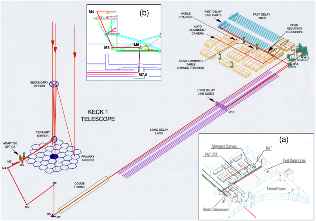
Fig. 1. Isometric view of the KI beam line from the Keck I side. Light propagates from the telescope through the AO system, DSM, and the telescope’s coude train to a crypt beneath the telescope at the basement level. The crypt houses the final mirror of the coude train, M7, and fold mirror M8, which directs light through the coude tube in the telescope foundation toward the “fore” switchyard in the interferometry basement. Fold mirrors M9 and M10 direct the light to the long delay lines, and their output is reflected toward the fast delay lines via mirrors M14. The output of the fast delay lines is compressed in diameter and directed into the beam combiner area, which includes the “aft” switchyard which feeds the fringe and angle trackers, nuller, and the back-end autoalignment cameras. Inset (a) show the first-light instrumentation, and illustrates the partitioning of space between the environmentally-controlled control room and rest of the beam-combining laboratory; the latter is partitioned with modular cleanrooms into a long delay line and beam transport area, a fast delay line area, and a beam-combiner area. Inset (b) shows the location of the coude mirrors on the telescope structure; the M4, M6 and M7 coude mirrors are 229 mm diameter, and the M5 mirrors, used at a larger angle of incidence, are 305 mm diameter.
While the interferometry control room has standard environmental controls, passive thermal control is relied upon for the beam combining lab. To attenuate environmental disturbances, the overall space was partitioned using modular Plexiglas cleanrooms into three rectangular spaces (see Fig. 1a): an LDL and beam transport area, as an extension of the coude tunnel between the two telescopes; an FDL area; and a beam combiner area. The latter two areas include panels above the spaces to provide further isolation from facility equipment (and from the small amount of make-up air provided near the back end), and also include access corridors outside of the cleanroom space. The coude tubes were also capped with optical windows, and various air leaks sealed, to minimize air flow within the interferometry basement. The LDL and FDL areas are largely free of electronic heat sources in order to limit induced turbulence; for example, the lasers and sensors used for the FDL metrology are fiber-coupled from the control room. There are more electronics along the periphery of the beam combiner area, but the small-diameter compressed beams (see § 2.1.4) and shorter propagation paths in that area (as well as the actual location of the electronics) limit their impact on beam-train seeing.
Figure 2 shows a plan view centered on the beam combiner area showing the final instrumentation complement. The outputs of the FDLs, after beam compression, are directed to the aft switchyard, where successively shorter wavelengths are extracted for the 10 μm nuller; the L-band or K/H-band fringe tracker(s); the H/J-band angle tracker; and the visible alignment system at the back end. The wavelength hierarchy isn’t strict due to the requirements for laser metrology and alignment. For example, the dichroic beamsplitter extracting light for the fringe tracker also needs to be partially reflective in the visible to support laser metrology and boresight functions. More detail on the overall optical configuration is given in § 2.5.
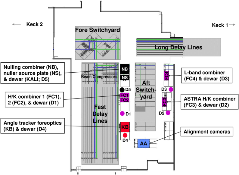
Fig. 2. Plan view of the beam combining laboratory showing the final instrumentation complement, including the three H/K beam combiners feeding two dewars; the L-band combiner and dewar; the 10 um nuller and dewar; the J/H angle tracker and dewar; and the back-end alignment cameras. The aft switchyard contains a number of deployable dichroics to feed the various instruments.
Standard optical tables are used throughout the facility to support the interferometer hardware. Because of the need to maintain stable alignment over a large and distributed facility, limited isolation of the interferometer optics from man-made disturbances is possible. Rather, isolation and suppression on the source side was implemented, along with selective stiffening and damping of interferometer components, and active control and feedforward as discussed in § 2.11. The large machines needed to support the Keck telescopes produced significant vibrations, and major efforts were made early in the interferometer project to reduce the influence of these vibrations (especially from large induction motors with tones at ∼29 Hz and ∼58 Hz) on the interferometer hardware (Hess et al. 2003). These mitigations included the seismic isolation of machinery, air handlers, and fluid lines; the use of damping on the hydrostatic bearing oil system and on the transport optics; and operations policies on the status of equipment during observing. The vibration environment improved over time as old machines were replaced with new machines with specific attention paid to vibration and isolation issues. In conjunction with active measures, these improvements led to more stable visibilities, and allowed the use of longer integration times. More discussion on vibration mitigation and final performance is given in § 4.3.
2.1.4. Pupil Management, Beam Walk, and Dispersion
As the KI science instruments are all single mode, for simplicity of implementation a collimated beam is propagated from the pupil at the deformable mirror in the AO system to the interferometer back end without any explicit pupil reimaging. This design affects the selection of the compressed beam diameter, the beam-train clear aperture, and the strategy for control of differential chromatic refraction (DCR).
The demagnification from the effective 10 m Keck aperture10 to the pupil on the deformable mirror is 80.4, so the starting beam diameter is 124 mm. A clear aperture (CA) of ∼150 mm is maintained for propagation at this diameter; the propagation distance in this space is typically 125 m, although it can vary by -45 m to +35 m depending on the LDL and FDL positions.
After 4:1 beam compression at the exit of the fast delay lines to 31 mm diameter (and for which a 44 mm CA is maintained), the propagation distances to the FATCAT fiber coupler, KAT, and the auto alignment system are 10.5, 14, and 16 m, respectively. Including this additional distance, the effective propagation distances, L, referred to the 124 mm beam diameter, d, are 290, 350, and 380 m, respectively.11 Thus, for K band, the Fresnel number d2/(4λL) at the beam combiner is 6.0, which is still within the geometric-optics limit. For the nuller, the propagation distance for the compressed beam to the 20 mm cold pupil stop in the nuller camera is 12 m, for L = 320 m, and a Fresnel number of 1.2: smaller than desired, but a compromise that greatly simplified the implementation.
The other aspect of the pupil management strategy is control of DCR between the angle tracking and science wavelengths. The angular dispersion attributable to astronomical refraction at Mauna Kea at a 45° zenith angle (ZA) is given in Table 1. Refraction is accommodated with a Risley prism pair at the input to the angle tracker. It is configured for the wavelength difference between fringe tracking and angle tracking in order to maintain a fixed alignment on the fringe tracker at the expense of beam walk on the angle tracker. The Risley prism pair differential angle tracks the telescope elevation, while the common angle tracks the telescope azimuth to account for pupil rotation. For J-band angle tracking and K-band fringe tracking at a 45° ZA, the beam walk on KAT computed using the propagation distance above is 3 mm for the 31 mm beam, which is accommodated in the design CA. The reverse calculation, allowing for beam walk equal to ½ of the CA, gives the usable acquisition FOV at the angle tracker of approximately ± 0.65″.
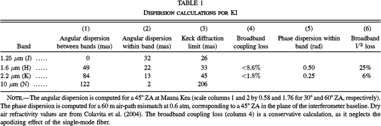 |
Table 1 also includes the broadband coupling loss attributable to image elongation, which is < 2% at K band. For the angle tracker, the image elongation causes a small amount of S/N degradation at large zenith angles, although the effect is usually masked by image residuals attributable to imperfect wavefront correction; systematic aspects are accommodated by our per-star flux optimization procedure (see § 3.2). Finally, the table includes the magnitude of the broadband longitudinal phase dispersion computed for a near worst-case delay of 60 m (45° ZA in the plane of the baseline). The broadband V2 loss is ∼25% and ∼6% at H and K band, respectively, and is quadratic with delay and with the number of spectral pixels. We absorb the small S/N impact, and account for the effect in the broadband channel through the usual target/calibrator observing sequence (see § 3.3.3). For the spectrometer channels at all of the provided resolutions, the effect is small.
2.2. Telescopes and Adaptive Optics
The two Keck telescopes are located on the summit of Mauna Kea, Hawaii, at 19.8° latitude and 4200 m elevation. The two altitude-azimuth telescopes are separated by 85 m, with the baseline oriented 38° east of north.12 Each telescope consists of 36 hexagonal segments. The 1.8 m (outer diameter) × 75 mm (thick) segments are each supported by a whiffletree support structure and a central radial post. The segments are actively controlled in piston, tip, and tilt using three actuators with feedback from capacitive sensors between neighboring segments in order to keep the primary mirror in phase and the segments stacked. The primary mirror has an outer diameter varying from 9 m (inscribed) to 10.95 m (circumscribed), and has the equivalent collecting area of a 10 m circular aperture. The central obscuration produced by the top end module is ∼2.4 m in diameter. The telescope’s primary, secondary and tertiary mirrors are all aluminum coated. The output focal ratio of the telescope at the left Nasmyth platform where the AO system is located is f/15 (assuming a 10 m equivalent aperture).
Each Keck telescope is equipped with an adaptive optics (AO) system. These are used for science with multiple science instruments in both natural guide star (NGS; Wizinowich et al. 2000) and laser guide star (LGS; Wizinowich et al. 2006b; van Dam et al. 2006; Chin et al. 2012) modes. The interferometer has only used the AO systems in NGS mode with the exception of the first science observations with LGS mode in 2012 July as part of the ASTRA program (preparations for these observations are described in Woillez et al. 2012b).
A schematic of the AO bench and interferometer dual star module (DSM) in the AO enclosure is shown in Figure 3. The AO bench and DSM are located within a thermally insulated clean room; personnel wear cleanroom garb for entry, and HEPA filters operate while people are within the room and when the system is not being used for observations. Heat sources are largely kept out of this cleanroom area. The AO and DSM electronics are thermally isolated within a neighboring electronics room. A hatch within the elevation ring is opened for AO observations. Two hatches located below the DSM feed light along the primary and secondary coude beam trains
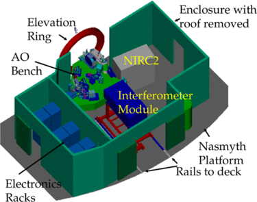
Fig. 3. Schematic view of the AO enclosure showing the interferometer dual star module next to the AO bench. Light from the telescope enters through the elevation ring along the telescope’s elevation axis. The AO enclosures are located on the left Nasmyth platforms of each telescope. In order to exchange AO instruments, the interferometer dual star module is stored on the Nasmyth deck and is transported into the AO enclosure with a motorized cart via rails and then lowered onto kinematic defining points.
A schematic of the AO bench is shown in Figure 4. The derotator (item 1) can be used to maintain either the field or pupil fixed. Both configurations have been used for the interferometer. Fixed-pupil is required by the nulling mode to allow the pupil split in the DSM; fixed-field is required by the DFPR mode to allow use of the AO field-separator mirrors. The other KI (full-pupil) modes can use either rotator configuration. The deformable mirror (DM; item 4) is a 349 actuator mirror from Xinetics. The primary is reimaged onto the DM such that 56.25 cm corresponds to the 7 mm actuator spacing. The Shack-Hartmann AO wavefront sensor uses the visible light below 1 μm.
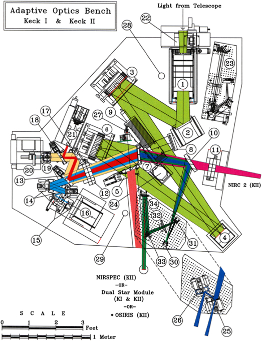
Fig. 4. AO bench schematic. Light from the telescope enters from the top of the diagram through derotator (1). A fast tip-tilt mirror (2) reflects the field to an off-axis parabola (3) which reimages the telescope primary mirror onto the deformable mirror (4). A second off-axis parabola (6) reconverges the light with the same f/# and pupil location as the telescope. The visible light for the wavefront sensor camera (16) is reflected off an infrared transmissive dichroic (7). Near-infrared light to the interferometer’s dual star module is reflected by a dichroic beamsplitter (5) in collimated space, or by a pair of field selector mirrors (25, 26), the first of which (25) is an annular mirror that passes the on-axis starlight.
For KI, the output of the AO system is directed to the DSM, which can be fed in two different ways depending on the mode of the interferometer. Originally both the V2 and nulling modes were fed from collimated space by an infrared reflective dichroic beamsplitter (item 5) that transmitted the visible light needed for the AO wavefront sensing and acquisition. The beamsplitter was upgraded in 2005 to provide improved throughput to the wavefront sensor from 0.7 to 1.0 μm for enhanced sensitivity when observing cool objects (at the expense of a small amount of J-band reflectivity). The pupil diameter exiting the AO system is 124 mm, for a demagnification with respect to the 10 m effective telescope aperture of 80.4:1
Subsequent to 2010 April, most interferometer modes, except for nulling, have been fed using a pair of field selector mirrors. An optical table containing these two mirrors is installed on kinematic supports on the AO bench for interferometer observations, as shown in Figure 4. The first field selector is an annular mirror (item 25) which transmits the on-axis light to the primary beam train of the DSM. The first and second field selector mirrors steer together to send an off-axis star within a 30″ diameter field to the secondary beam train of the DSM.
All of the AO bench mirrors in the path to the DSM have protected silver coatings, with the exception of two of the three derotator mirrors. Because of their steep incidence angles, these are coated with aluminum to avoid mid-infrared polarization effects which can occur with protected metal coatings (see Hass 1982). The two beamsplitters are fused silica (item 5) and calcium fluoride (item 7).
The AO control system includes several accommodations to support interferometry. In particular, low bandwidth pointing corrections (implemented via offsets to the centroid targets) allow for offloading the back-end angle-tracking errors, and an offset capability using the AO field-steering mirrors allows for coarse alignment of the AO output to the interferometer beam train. In support of nulling alignments, a synchronized narrow-angle chopping mode was added. This mode is implemented via simultaneous feedforward to the AO tip-tilt mirror and to the WFS centroid offsets to provide fast transitions, with AO feedback correcting for residual scale-factor errors. Two patterns are supported: a two-sided chop, typically ± 0.15″, and a “four-sided” chop (+x, 0 - x, 0, +y, 0, -y, 0), typically ± 0.25″, both typically at 5 Hz. While the nuller gets its photometry from the fringe amplitude on the short cross-combiner baseline, this chopping capability is used on bright stars to align the nuller FOV between observation clusters.
2.3. Dual Star Module
The dual-star module (DSM) relays light from the Keck AO system to the telescope coude train for propagation to the interferometry basement.
The DSM is built on a custom optical table mounted to a handling cart, allowing it to be rolled from its storage location on the Nasmyth deck along rails into the AO enclosure as shown in Figure 3. The 124 mm beam from the AO extraction dichroic is relayed from the AO bench enclosure into the DSM table enclosure as shown in Figure 5. For V2 operation, optic M2-P is a simple fold, directing all of the light toward M3-P, and the secondary optics are not used. For nuller operation, optic M2-P is a half mirror, which sends the left half of the pupil toward M3-P and the right half toward M3-S; the vertical edge of the mirror is carefully aligned to the center of the AO DM, which is the true system pupil. The two M3 optics are dichroics (hot mirrors), transmitting HeNe at 633 nm and reflecting longer wavelengths. The two M4 optics are fold mirrors which direct light down and toward the coude train’s M5 optics. A combination of commercial and custom mounts is used to fit the tight space and to allow for remote actuation. A 150 mm CA is maintained, as previously described, with fold mirror M4 using a gold coating, and M2, used near normal incidence, using protected silver.
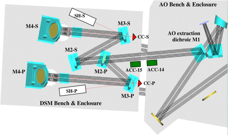
Fig. 5. DSM schematic, showing the starlight path from the AO extraction dichroic M1 (item [5] in Fig. 4) through to the coude-injection folds M4-P and M4-S. CC-P and CC-S are corner cubes which serve as the endpoints of the laser metrology, visible through the M3 dichroics. ACC-14 and ACC-15 are accelerometers attached to the optical benches; ACC-13, not shown, is attached to the other side of the AO bench, beneath the image rotator, aligned with the input from the Keck telescope tertiary. The usage of accelerometers is described in § 2.11. The shear sensors SH-P and SH-S, used for nulling operations, are fed via beamsplitters between M3 and the metrology corner cubes, reflecting back through M3. Not shown are shutters and CCD cameras used for alignment.
The corner cubes CC-P and CC-S, located behind the M3 dichroics, serve as the end points for the coude metrology described in § 2.11. To support nuller operation, two shear sensors are also located on the DSM bench, shown schematically in Figure 5. They are fed via partially-reflecting beamsplitters located between the M3 mirrors and the corner cubes. The shear sensors image the inner 65 mm of the back-propagated pupil onto small CCD cameras. By measuring the lateral position of the boresight pencil beam propagated from the interferometry basement, the shear sensors enable accurate alignment of the system pupils to minimize nuller leakage errors attributable to beam shear. The shear sensor also includes an intermediate relay, which can be used to inject a collimated reference beam into the beam train toward the interferometry basement.
This DSM configuration was used for the majority of interferometer operations. However, as discussed in § 2.2, after completion of the nuller science program, the DSM was reconfigured as part of the ASTRA program to include recollimating optics in order to use the focal output of the AO system, and most V2 data obtained after 2010 April were taken in this configuration
2.4. Coude Train
Figure 1b shows the locations of the coude mirrors on the lower portion of the Keck telescope structure. Two mirrors are mounted at each of these locations, one each for the primary and secondary beam trains. The two M4 mirrors are located on the interferometer DSM. Holes in the floor of the AO enclosure and Nasmyth platform transmit light to the two M5 mirrors. The M4 and M5 mirrors are manually positioned, as are the primary M6 and M7 mirrors. The primary M6 and M7 mirrors are used as a classical on-axis coude train, and the beam between these two mirrors runs along the telescope’s azimuth axis. However, the secondary M6 and M7 mirrors are both located off the azimuth axis and must therefore track as the telescope rotates. With respect to starlight, the control system points M6S to locate the pupil on M7S, and points M7S to maintain a fixed output direction, using an azimuth-dependent pointing model. This control system, as with the AO system, accommodates low-bandwidth pointing corrections to allow for offloading back-end angle-tracking errors.
Mirrors M7P, M7S, M8P, and M8S are located on a small optical table in a “crypt” beneath the telescope; a remote hatch keeps the space sealed between observing runs (a remote hatch also helps keep the up-looking M5P and M5S mirrors clean between runs). To maintain proper image rotation between Keck I and II, the reflection from M7 is at 90° to the interferometer baseline, with M8 directing the light into the beam combining lab. In conjunction with the folds from transport optics M9 and M10, this configuration provides matched image rotation at the input to the LDLs. The exit from the crypt into the coude tube is via a pair of optical windows: Infrasil is used for near-infrared observations and ZnSe for nulling observations. These windows eliminate air flow from the domes into the beam combining laboratory. The coude tubes from the crypt into the beam combining lab are 1 m diameter × 15 m long. Because of the close proximity of the starlight beams to the walls of these tubes, their inside walls are insulated.
2.5. Beam Transport and Long Delay Lines
After exit from the Keck I and Keck II coude trains, the 124 mm primary and secondary beams, arranged vertically, 176 mm center-to-center, are directed to the fore switchyard on a high-rise assembly as shown in Figure 1, where mirrors M9 and M10 fold the beams toward the long delay lines (LDLs).
All of the transport mirror mounts, including the LDL flats, are of a similar, compact, elevation-over-azimuth design, with rotational flexure bearings used for elevation rotation, and four blade flexures arranged circumferentially beneath the elevation assembly to provide limited azimuth rotation. DC-motor micrometers (modified Newport 850G actuators) drive the axes directly (elevation) or via a flexural lever (azimuth). Certain mounts include viscous (shear) dampers to minimize response to environmental disturbances. The optics are rectangular Zerodur flats sized to maintain the clear aperture. All normal incidence mirrors use protected silver coatings, while 45° reflections use bare gold; protected silver coatings are used both at normal and 45° incidence elsewhere in the beam train that see only near-infrared light (see the coating discussion in § 2.2). While the transport mounts remain energized during observations to maintain actuator encoder readings, most do not actively track, and a dead zone in the control ensures that the servo is disabled at completion of a move.
The LDLs use double-height transport optics which can be positioned along rails with a usable travel of 36 m, for a delay range of 0 to 72 m. Because the beam combining laboratory is toward the K2 side of the facility, zenith pointing requires the K2 LDL back ∼20 m with respect to the K1 LDL, providing ∼40 m of delay on the K2 side. A schematic of the LDL is shown in Figure 6. The optics cart is driven by a large stepper motor with an optical encoder via a rack and pinion drive.13 Guidance is provided by a 38 mm round rail and two pairs of cam followers, with a flat rail and a single cam follower on the other side to complete the support. Unlike the FDL, the LDL is “move-and-clamp,” i.e., it is stationary during observations, so that smoothness of motion is not paramount. Thus the tractor motor is mounted directly to the optics cart. An idler cart manages the cable that powers the LDL, and a motorized reel tensions the idler cart. The LDL drives are only energized during moves, with the cart’s position maintained by a brake on the drive shaft.
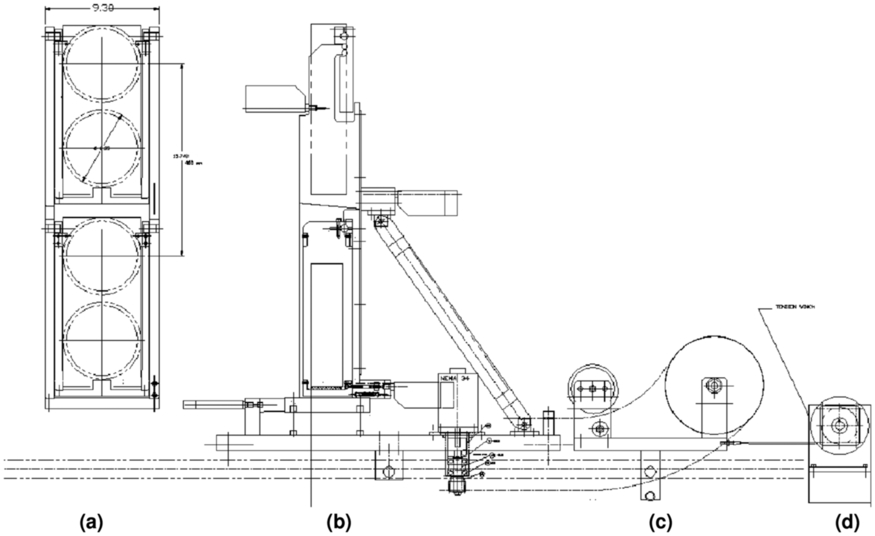
Fig. 6. Schematic of the long delay line cart. From left to right: (a) front view showing the beam footprints (only the top mirror position is used); (b) side view of the main cart with its tractor motor; (c) the idler cart, shown for the LDL at the back; (d) the tensioner motor.
As the LDL uses a flat mirror, and not a cat’s eye, it is necessary to adjust the tilt of the LDL injection mirror (M10; see Fig. 1) and the LDL flat (M11) as a function of delay. A lookup table is used for coarse adjustment of these mirrors in order to stay within the FOV of the alignment system; subsequent fine alignment is done using starlight sensed by the angle tracker. In addition to accounting for basic geometry (viewed from the side, M10 folds the beam down toward M11, while M11 folds the beam to exit horizontally ∼400 mm below the centerline of M10), the lookup table accounts for measured tilt errors from rail irregularities.14 The overall controller also positions the cart to account for the LDL geometry, as the delay is slightly longer than twice the longitudinal cart position. The slight elevation tilt of M10, which is otherwise a simple right-angle periscope, breaks the strict image-rotation symmetry of KI. However, the differential rotation is typically smaller than 2° (less when the LDLs are toward the back), and since the effect on visibility is quadratic, the net impact is small.
After exit from the LDLs, the beam pairs are directed toward the M14 mirrors15 as shown in Figure 1. The primary M14 mirrors extract the lower beams and direct them toward the primary FDLs through apertures in the cleanroom walls. Similarly, the secondary M14 mirrors, behind the primary M14 mirrors, and 176 mm higher, extract the upper beams and direct them toward the secondary FDLs. The M14 mirrors include PZT actuators, used for low-bandwidth angle tracking (see § 2.9), as well as for quasistatic adjustments to beam shear in conjunction with the shear sensors on the DSM.
For full-aperture V2 observations, only the two primary FDLs are used. For split-pupil (nulling) mode or dual-star (ASTRA) mode, the two secondary FDLs are also used. For nulling mode, dichroic beamsplitters (K/N splitters) are rotated into place in front of these four FDLs. The K/N splitters transmit the near-infrared and reflect the N-band light to fold mirrors (N-folds) to feed two additional primary and two additional secondary FDLs, as illustrated in Figure 7. The K/N splitters, which are actually beamsplitters in the near-infrared, are also used on the primary side in the ASTRA self-phase-referencing (SPR) mode, splitting the near-infrared light between the primary FATCAT (via FDLs 1 and 2) for cophasing, and the ASTRA science combiner (via FDLs 3 and 4) for high spectral resolution measurements.
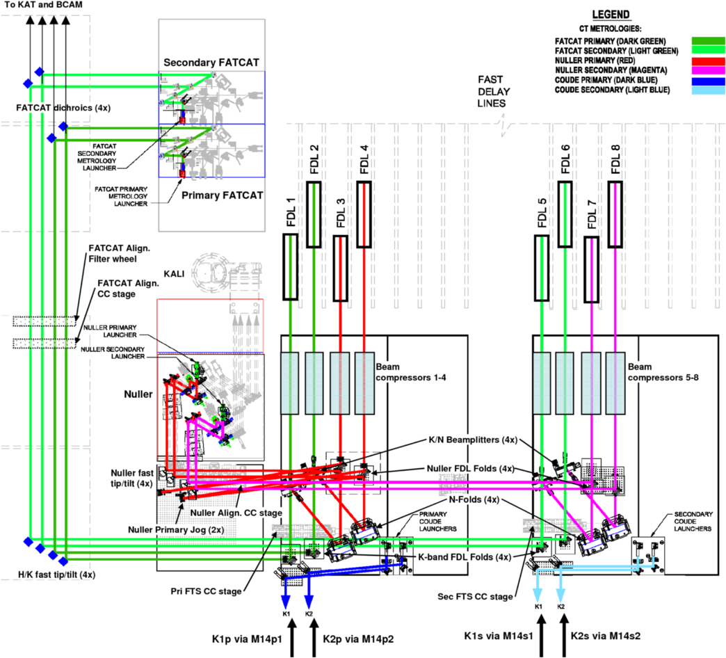
Fig. 7. Schematic of the FDL injection and extraction in nulling mode, and the fore switchyard through to the FATCAT dichroics. Starlight from the primary and secondary beams enters via reflection off of the M14 mirrors. The K-band light transmits to FDLs 1, 2, 5, & 6, and the N-band light reflects off the K/N beamsplitters and N-folds and is directed to FDLs 3, 4, 7, & 8. The output of the K-band FDLs is directed toward fast tip/tilt mirrors and then to the primary and secondary FATCATs (and KAT—not shown). The output of the N-band FDLs is directed toward the nuller fast tip/tilt mirrors and then to the nuller breadboard; the path from the primary nuller delay lines includes an extra path-length jog to partially equalize the path lengths from the primary and secondary delay lines in order to better utilize the FDL range. Also shown are the primary and secondary coude metrology launchers, as well as the CT metrology launchers which were used for initial nuller cophasing characterization, as discussed in § 2.11. Also shown are slide-in corner cube stages used for internal fringes and for alignment, as discussed in § 2.13.
As shown in Figure 7, after exit from the FDLs, the beams are compressed by 4:1 to 31 mm diameter with off-axis Dahl-Kirkam beam compressors, and are folded toward the beam combining laboratory in the adjacent modular room. The near-infrared beams from FDLs 1, 2, 5, and 6 (or 1, 2, 3, and 4 for ASTRA SPR) are directed toward fast tip/tilt mirrors which fold the beams down the length of the aft switchyard. The fast tip/tilt mirrors use light-weighted flat mirrors attached via flexures to PZT tip/tilt stages (PI S330), allowing high bandwidth pointing corrections from KAT. The 10 μm beams from delay lines 3, 4, 7, and 8 are directed toward fast tip/tilt mirrors that feed the nuller; these mirrors, whose motion is not sensed by KAT, are slaved to the near-infrared fast tip/tilt mirrors.
Progressing down the aft switchyard (see Figs. 7 and 2), dichroic beamsplitters extract fringe-tracking light at H/K, K, or L band, depending on the configuration. The reflected light is sent to the primary FATCAT for standard V2; the primary and secondary FATCATs for nuller cophasing; the L-band FATCAT for full-pupil L-band V2; the L-band and primary FATCATs for dual-wavelength split-pupil mode; or the primary and ASTRA FATCATs for self- and dual-phase-referenced modes. These H/K and K dichroics are also partially reflective over the visible band between 630 and 660 nm for use with the metrology and boresight lasers, and have sufficient out-of-band leakage to enable alignments involving KAT at J and H, and the auto alignment cameras in the visible.
Beyond the fringe trackers, a second set of dichroic beamsplitters extract the J/H light for angle tracking with KAT, while the visible light is transmitted to alignment cameras at the back end of the beam train (see Figs. 1 and 7). Also shown in Figure 7 are three sets of corner cube translation stages, one set located in front of the FDLs and used for FTS testing; another located between the fast tip/tilt mirrors and the FATCAT dichroics used for FATCAT and KAT alignment; and a third set located at the input to the nuller used for nuller alignment.
2.6. Fast Delay Lines
The Fast Delay Lines (FDLs) used on KI are similar in principle and implementation to those used on PTI (Colavita et al. 1999). KI uses eight FDLs: two are used for single-star V2 observations, four are used for SPR and the split-pupil V2 modes, and all eight are used for nulling and DFPR modes. The usable physical delay line travel of each FDL is 7.5 m; both delay lines in a pair are active when observing, providing a delay range of ± 15 m.
2.6.1. Opto-Mechanics
As shown in Figure 8, a simple cat’s eye assembly is implemented using a 1077 mm focal length parabola and a 12.5 mm diameter flat mirror. Focus is maintained with invar spacers and shear panels, and protected silver coatings are used on the optics. The starlight beam input and output are arranged vertically, 176 mm center-to-center, and the parabola is cut to a rectangular shape, allowing close packing of 275 mm between delay lines. The flat mirror is mounted on a custom piezoelectric (PZT) actuator consisting of a preloaded series assembly of a 25 μm stroke PZT (-10 to +150 V) for servo control and an 8 μm stroke PZT for fringe demodulation (a.k.a. dither). Separate PZTs are used such that the fringe demodulation—programmed open-loop via a lookup table—remains unaffected by PZT nonlinearities as the servo PZT responds to the control system. A second PZT is mounted on the front of the FDL cart in opposition to the first for momentum compensation. A dust cover helps keep the PZT mirror clean, as the starlight and metrology light are focused on its surface, and flexible magnet panels cover the access holes in the invar shear plates.
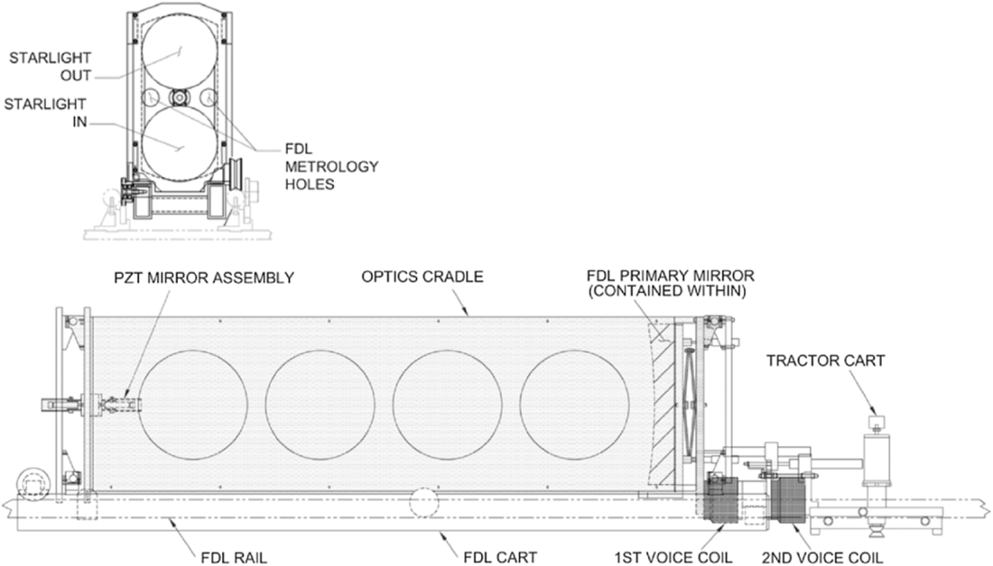
Fig. 8. Fast delay line cart. As shown in the top panel, the input and output beams are arranged vertically, and the metrology apertures are arranged horizontally. The lower panel shows a side view of the optics cart and the tractor cart. An idler cart (not shown), tensioned by a spring reel, manages the ribbon cable that provides power to the FDL.
The cat’s eye assembly is supported on a three-wheeled optics cart using a four-bar linkage implemented with rotational flexures. The optics cart uses two 75 mm vee-wheels on one side riding on a 38 mm round rail for angular guidance, and a single 60 mm wheel on the other side riding on flat rail to complete the support. A voice coil motor drives the cat’s eye assembly with respect to the optics cart. The relative position is sensed with a linear variable differential transformer (LVDT) sensor, and a composite coil form is used in the voice coil motor to minimize eddy current damping. The optics cart is driven via a second voice coil motor from a separate tractor cart shown on the right in Figure 8; the relative position of the optics and tractor carts is measured with a second LVDT (this one with an internal bearing). The tractor drive uses a micro-stepped stepper motor with an inertia damper coupled through a 5:1 gearbox to a 25 mm vee-wheel which drives against a central 25 mm drive rail. FDL drive and sense power is via a ribbon cable which runs in a plastic tray adjacent to the drive rail. The cable is managed using an idler cart that is preloaded using a passive spring-reel cable tensioner. A precision magnetic home switch (Sony Magneswitch) attached to the cat’s eye assembly provides a micron-repeatable zero point. The track straightness (both lateral translation and tilt) limits beam shear to ∼2 mm over the range of delay line travel.
2.6.2. Metrology
The delay line positions are monitored using standard heterodyne metrology, as widely used in optical interferometers (see Shao et al. 1988). The laser source plates use stabilized (10 ppb) 633 nm HeNe lasers and acousto-optic modulators (AOMs) with a 2 MHz frequency difference. The source plates are located in the KI control room, and feed their s- and p-polarized outputs using separate single-mode polarization-maintaining fibers to 1:4 fiber splitters into the laboratory area. These fiber splitters feed fiber-coupled beam launchers as illustrated in Figure 9. The metrology launchers, and corresponding retroreflectors mounted in front of the delay lines in the vertical gaps between starlight beams, are used to measure the FDL optical paths in double pass; the metrology apertures on the front plate of the cat’s eye assembly are shown in Figure 8.
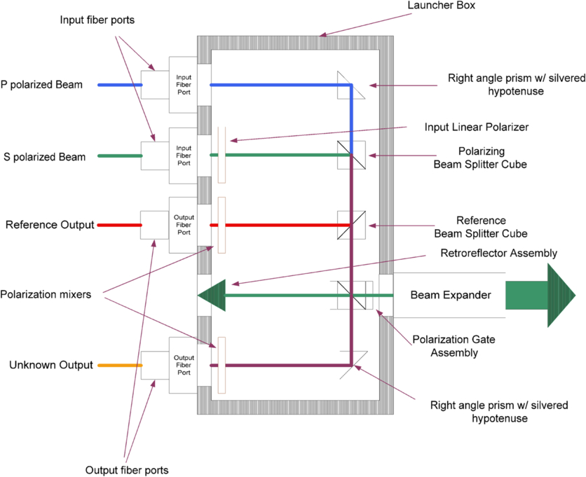
Fig. 9. Metrology beam launcher. The launcher implements a standard heterodyne metrology gauge. Input s- and p-polarized beams are provided via separate single-mode polarization-preserving (SM) fibers, collimated, and combined at the top of the figure; the extra polarizer on s-polarized beam, which reflects from the polarizing beamsplitter cube, improves the polarization quality of the combined beam. A reference beam is extracted, sent through a 45° linear polarizer, and output via a multi-mode (MM) fiber to electronics in the computer room. The “unknown” beam measures the distance between the internal reference retroreflector and an external retroreflector using one polarization, is combined with the other polarization, sent through a 45° polarizer, and output through a second MM fiber. For use as a CT-metrology launcher (see § 2.11.3), the polarization gate assembly (a polarizing beamsplitter cube with two quarter wave plates) is replaced by a single nonpolarizing beamsplitter cube so that both the s and p polarizations are directed out through the beam expander; the internal retroreflector is removed; and the output fiber coupler and polarizer moved up to the retroreflector location to collect the returned light.
The optical output of the launchers—reference and unknown signals—are returned to the computer room using multimode fibers where they feed fiber-coupled preamps followed by an automatic gain control (AGC) stage16 and comparator. The fringe phase is quantized in a digital laser-counter card to 7 bits, and as the metrology is double pass with respect to the starlight, provides a delay resolution of 1.2 nm.
2.6.3. Control Aspects
The delay line is fully programmable in position and rate, and includes a target generator (500 Hz update) to generate smooth trajectories from low rate inputs such as sidereal targets.
In track mode, four nested control loops are implemented:
- 1.PZT loop (4 kHz update): This loop implements PD (proportional-derivative) control of the PZT rate via a digital integrator connected to a digital-to-analog converter (DAC) which feeds the amplifier for the servo PZT. The servo error is computed from the current target trajectory and laser metrology feedback; delay line targets requiring low latency can bypass the target generator and feed the PZT loop directly.
- 2.Optics voice coil loop (800 Hz update): This loop uses the PZT position read back from the digital integrator (and includes an additional feedforward from the servo error to maintain stability in the event of PZT saturation) and implements PID (proportional-integral-derivative) control of the optics voice coil to continuously offload the PZT. The optics voice coil force is compensated by adding a feedforward of its command to the tractor voice coil servo output to prevent reaction of the optics cart.
- 3.Tractor voice coil loop (800 Hz update): This loop uses the optics voice coil position as measured by its LVDT sensor and implements PID control of the tractor voice coil.
- 4.Motor loop (100 Hz update): This loop uses the tractor voice coil position as measured by its LVDT sensor and implements PD control to update the motor rate; the mean motor rate is provided as a feedforward from the target generator.
For large moves, the FDL controller switches to slew mode, which disables the PZT loop, stabilizes the two voice coils using their collocated sensors, and drives the motor using the servo error. The delay slew rate must be kept less than 0.6 m/s in order to keep the Doppler shift on the (double-pass) metrology to less than 2 MHz.
The controller also implements several calibration functions, including home set/check to clear/read the metrology position at the fiducial mark, and a dither-calibrate function. The latter creates a position lookup table that accounts for non-linearity and hysteresis of the dither PZT to generate the triangular waveform for fringe demodulation; high time resolution to provide good waveform fidelity is accomplished through varying the phase of the interrupt clock used by the FDL control system.
2.6.4. Performance
The two fastest loops are usually tuned for ∼800 Hz and ∼25 Hz command bandwidths, respectively. Based on measured error rejection versus frequency, the effective command latency is 0.7 ms, providing disturbance rejection below 250 Hz. For feedforward commands from external metrology and accelerometers, provided directly to the PZT loop, a lead filter is implemented to improve mid-frequency rejection at the expense of increased peaking above 300 Hz, where there are typically only limited disturbances, achieving 20 dB suppression at 90 Hz. See § 2.7 for discussion of the performance of the FDL as used with the fringe tracker.
2.7. H/K-Band Fringe Tracker
The H/K-band fringe tracker, FATCAT (“Fast Atmospheric Tracking Camera At Two-microns”; Vasisht et al. 2003), is used as a primary science instrument for V2 measurements as well as to provide cophasing for observations in the nulling and ASTRA modes. It operates at H and K bands with frame times down to 4 ms. It incorporates free-space beam combination optics with single-mode fiber inputs to an infrared dewar. KI has three H/K FATCATs as shown in Figure 2: Two feed a single dewar, and a third, implemented as part of the ASTRA upgrade, feeds a second dewar.
2.7.1. Optics
Figure 10 shows the free-space combination optics, implementing a traditional Michelson beam combiner, similar to that used at PTI. It is fed from dichroic beamsplitters in the aft switchyard. It is optimized for the H and K bands, although the beamsplitter is usable in the visible to support metrology and alignment functions. The two beamsplitter outputs are directed into single-mode fibers with integral vacuum feedthroughs directly into an infrared dewar. No photometric channels are provided; calibration for flux imbalance is provided using interleaved single-aperture calibrations as discussed in § 3.2. The use of free-space combination, and post-combination fibers, allows more ready incorporation of end-to-end laser metrology.17
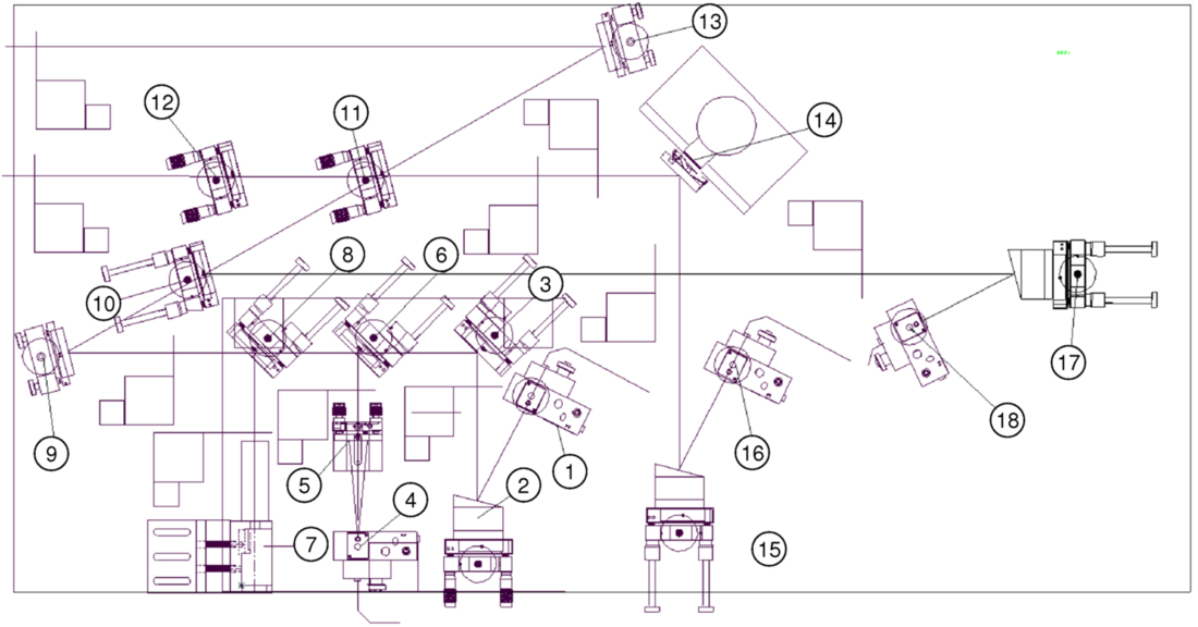
Fig. 10. FATCAT foreoptics breadboard. Light enters from the left. The main beamsplitter (11) is used with compensator (12). Optic (14) in series with one beamsplitter output is a raster mirror, which is used for optimizing coupling into the optical fiber via OAP (15) and fiber mount (16); a second raster mirror, not shown, is in series with the second fiber feed (17, 18). The FATCAT stimulus (1–9) is injected through the coupler (10: a leaky dichroic mirror), and includes a fiber-fed white light source (1) and a fiber-fed boresight laser (4) injected using a rugate beamsplitter (6). Item (7) is a metrology beam launcher used as discussed in § 2.11, which is injected via a second rugate beamsplitter (8). Also shown on the schematic are ten two-position shutters used during alignment as beam blocks or to insert pencil-beam irises.
The stimulus and alignment beams are introduced through a visible/IR dichroic fold mirror, which leaks slightly at H and K, to allow some infrared transmission. The stimulus includes a fiber-coupled tungsten-halogen white-light source, and a 658 nm single-mode fiber-pigtailed laser coupled into the combined beam with a rugate notch filter. A remote-actuated flip-in iris in the stimulus provides a pencil beam used for beam-train alignments. A second rugate notch filter in series with the white-light and laser stimuli can be used to inject the 633 nm constant-term metrology as discussed in § 2.11.
The fold mirrors directing light to the fibers are mounted on PZT tip/tilt stages (“raster mirrors”) and are used for optimizing coupling into the fibers. The fiber feeds use 81 mm focal length off-axis parabolas (OAPs) to couple light into custom fluoride-glass fiber assemblies (LVF IRguide-1: 6.5/125 μm; NA = 0.17; 1.45 μm cutoff) with integral vacuum feedthroughs. The mode-field diameter is 27.5 mm, which is close to optimal for a 31 mm beam, providing a theoretical coupling efficiency of ∼70% for the (obscured) Keck pupil. A separate, standalone white-light stimulus, which provides nearly uniform (vs. Gaussian) illumination over the starlight pupil, can be used to provide improved sensitivity for alignment of the fiber feeds.
2.7.2. Camera
The dewar optical schematic is shown in Figure 11. It uses a custom dewar with a 30 cm diameter cold plate, and two LN2 reservoirs connected to an autofill system, with an ion pump used to maintain good vacuum between observing runs. The vacuum segments of the four fibers are routed to fiber collimator doublets (19 mm diameter clear aperture; 70 mm focal length) which are mounted on PZT tip/tilt stages to adjust pointing onto the array. The four collimated beams are combined and reflected via a pyramidal mirror through a 5-position filter wheel and 5-position prism wheel, to a final camera relay (50 mm diameter; 84 mm focal length) onto the infrared array mounted directly behind the annular fold mirror. A cryomotor allows remote control of the focus of this final stage. The filter and prism wheels are remote controlled via external motors and mechanical feedthroughs.
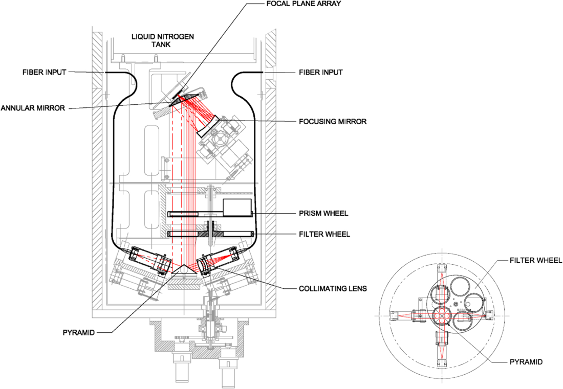
Fig. 11. FATCAT dewar. Light enters through four single-mode fibers. Each beam is separately collimated, and the four beams are multiplexed onto a pyramidal mirror, directed through filter and prisms wheels, and then imaged onto the infrared array. The position of the final focus mirror is adjustable using a cryo motor, and the filter and prism wheels are controlled via mechanical feedthroughs to external motors.
The filter wheel provides positions for H; K; K′, continuous H-K, and a split filter which provides a K filter for the two of the beams and is open for the other two beams. This latter configuration was most commonly used, with the K side used for the broadband channels, the open side used for the spectrometer channels. For the typically fast readouts used, any background penalty from the lack of a filter in the open channel was made up for by the higher transmission. The prism wheel provides, for two of the four beams (corresponding to the open half of the split filter setting), narrow- and wide-deviation direct-view prisms, and for one of the four inputs, a medium-resolution grism. At K band, the prisms and grism provide 5, 10, or 42 pixels across the band, with the ASTRA version, which includes a high resolution grism, providing 330 pixels across the band for SPR observations. At H band, the wide deviation prism is used providing 4 pixels across the band. The wavelengths are determined from FTS measurements.
FATCAT uses one quadrant (512 × 512) of a Rockwell HAWAII HgCdTe 1024 × 1024 infrared array with a 2.5 μm cutoff. Using the PZT adjusters on the collimating lenses, each spot or dispersed spectrum is arranged onto one 18.5 μm pixel, or onto one row of pixels, to minimize the required number of pixels that must be read; multiple nondestructive reads of each pixel are used to further reduce noise. The PZTs on the collimating lenses are adjusted using the FATCAT stimulus seen in retroflection through a narrowband filter to provide repeatable spectral alignment (see § 2.13). The usable flux per frame per pixel is ∼60,000 e- in order to keep V2 errors attributable to array saturation to < 0.3%.
The array electronics are commercial (Leach & Low 2000), using a pre-amp attached to the dewar feeding an external post-amp and 1 MHz/16 bit digitizer (0.26 DN/e-). The output is connected via a custom fiber link to a custom clock control and interface card in the FATCAT VME chassis, which includes a downloadable waveform memory for the clock pattern, as well as an interface to the digitizer. A coadder provides hardware support for multiple nondestructive reads, and CDS read noise of 5 e- to 10 e- can be obtained for the low resolution modes where only a small number of pixel are read. While they may share a single dewar, from a controls perspective each beam combiner is logically separate.
In retrospect, the single-piece fiber assemblies generally worked well, providing a low-background dewar without the need for baffles and stops, avoiding losses from window transmission, and allowing for easy multiplexing of multiple inputs. The fiber assemblies survived multiple thermal cycles over the life of the instrument, and the few issues we encountered occurred only on the first cool-down. The tradeoffs for this approach are that pointing and focus inside the dewar required internal actuators, rather than allowing compensation from an external feed, and that the far end of the fibers were not directly accessible, so that fiber input alignment and optimization could only be done via readout of the array.
2.7.3. Control Aspects
In conjunction with path-length modulation on the delay line, FATCAT uses an ABCD algorithm to measure the fringe phasors. The fringe phase is used to command the delay lines to stabilize the optical path, and the fringe amplitude and phase are used for science measurements. When fringe tracking, FATCAT operates at frame rates of 4, 5, 8, or 10 ms, depending on the mode and seeing; when phase referenced for the ASTRA SPR or DFPR mode, much longer integration times are possible (see § 3.1). The fringe tracker has strong heritage to PTI, and algorithmic details and performance of the KI implementation are provided in a separate paper (Colavita et al. 2010a).
In low resolution modes, the white light (WL) and coadded spectrometer channels are coherently combined to increase the S/N for phase estimation via the usual ABCD algorithm, but implemented using a sliding integration window to decrease control latency. The phasors are corrected for mismatches between the dither wavelength and actual wavelength (‘‘dewarping”). In all modes, the spectrometer data are phase referenced to the WL phase—typically for 12 frames—to improve S/N before estimation of group delay via a coherent DFT algorithm.
Phase and group delay can be combined in different ways to generate the FDL control signal. For V2 operations, a simple fast inner phase loop with a slow outer group delay loop is employed. With a zero target to the outer loop, the servo asymptotically tracks to zero group delay while correcting fast phase fluctuations. However, to reduce V2 systematics that depend on phase (e.g., from a nonlinear dither), the target for the outer loop is typically configured as a low frequency triangle wave, one wavelength peak-to-peak, so that visibility measurements are averaged over 2π of phase.
A different servo loop, which tracks to a fixed phase point within the coherence envelope, is used for nuller and ASTRA cophasing. The system is optimized for low control latency in the cophasing path. Both the feedback and phase referencing paths include active control of narrowband disturbances (as does the feedback path for the V2 mode). In addition, a robust algorithm to estimate the slowly varying water vapor dispersion as required for nuller cophasing—essentially synthesizing a long coherent integration time on the dispersion only—was also implemented.
Transitions among search, semi-lock, and lock states use the fringe S/N estimated using a modified ABCD algorithm optimized for rejection of scintillation. The fringe search uses a geometric spiral about the last lock position. The transition to semi-lock is based on the instantaneous S/N exceeding a threshold, while the transition to and from lock depends on the average S/N. The threshold includes an additive term to set a minimum V2 floor in addition to a scalar S/N threshold.18
2.8. L-Band Fringe Tracker
The L-band fringe tracker (Ragland et al. 2009) has a similar architecture to the H/K-band system described in § 2.7. The free-space combiner implementation is similar to that in Figure 10, with the primary difference being in the optical substrates (CaF2 instead of Infrasil), coatings (different bandpasses for beamsplitters, switchyard dichroics, and couplers), and stimulus (IR emitter instead of a tungsten/halogen bulb). Post-combination optical fibers are also used, in this case a heavy-metal fluoride-glass fiber assembly (LVF IRguide-2: 8.5/125 μm; NA = 0.17; 1.9 μm cutoff; 0.15 dB/m at 4.2 μm). Coupling is via a 117 mm focal length OAP.
A custom dewar with a 35 cm diameter cold plate is used, similar to that shown in Figure 11, where the larger diameter allows better internal routing of the optical fibers. Only two ports are used, supporting a single L-band beam-combiner breadboard. Most observations used an L′ filter, although a KL filter was also available, along with a direct-view ZnSe/sapphire prism providing 10 pixels of dispersion over the band.19
The detector is a Rockwell HgCdTe PICNIC 256 × 256 FPA with a 5 μm cutoff and 40 μm pixels, of which one 128 × 128 quadrant is used. The PICNIC and HAWAII arrays have similar multiplexer architectures, allowing commonality of array control with the H/K system. Read noise through the electronics is typically 40–50 e- using multiple reads, with a scale factor of 0.065 DN/e-. In operation, shot noise from the background contributes a similar amount of noise.
Control of the L-band system is nearly identical to that of the H/K system. As both ports are dispersed for the L-band system, one port is coadded over the 10 pixels to provide a synthetic white-light channel, similar to the H/K system. Because of the longer wavelength, and corresponding longer atmospheric coherence time, longer frame times can be used, and the L-band system typically uses up to 20 ms frame times. Operationally, the main difference from the H/K system is that the background is significant, and the flux zero point must be measured by nodding off target, rather than through the use of a shutter in front of the fiber feed. Accuracy of the flux calibration adds an additional uncertainty to the V2 for faint objects as discussed in § 4.2.
2.9. Angle Tracker
The Keck Angle Tracker (KAT; Crawford et al. 2006) provides facility angle tracking at J and H band in support of all interferometer modes. It incorporates a fore-optics table that multiplexes inputs from four 31 mm beams to feed an infrared camera using a HAWAII HgCdTe array.
The plate scale on the array referred to the sky is 31 mas/pix. For comparison, the H-band aperture diffraction limit is 33 mas, and thus the system is not formally critically sampled. However, in practice the images are usually slightly larger due to imperfect AO correction at the shorter wavelengths, or residual aberration, and this scale factor works well, limiting the additional detector read noise that would come from finer sampling.
2.9.1. Optics and Camera
As shown in Figure 12, four dichroics reflect two primary and two secondary beams to fold mirrors on the KAT foreoptics table. These fold mirrors direct the four beams, on an approximate 75 × 150 mm grid, into a Cassegrain telescope with a parabolic primary (305 mm diameter; 914 mm focal length) and a convex spherical secondary (51 mm diameter; -125 mm focal length). The beams are deviated from the telescope’s optical axis such that their projections overlap ∼20 m front of the telescope; the telescope images this pseudo pupil close to the detector lens at a demagnification of 1.8:1. An apochromatic triplet (38 mm diameter; 101 mm focal length) produces four images on one quadrant of the detector array on an approximate 35 × 70 pixel grid for the array’s 18.5 μm pixels; the images are centered near a corner of a quadrant to enable rapid array readout. The quasi-pupil approach employed is scalable to a larger number of input beams. Remote-controlled shutters in front of the KAT fold mirrors and the dewar are used as part of the calibration process.
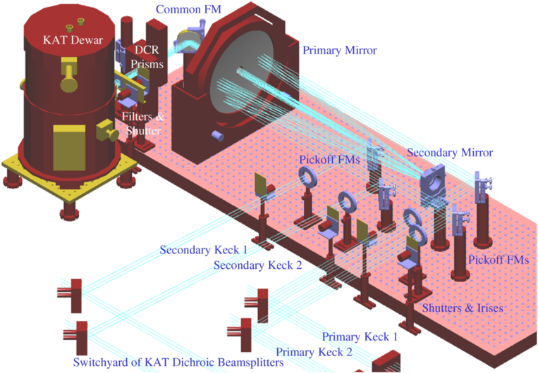
Fig. 12. KAT foreoptics and dewar. Four beams enter from the aft switchyard through the four alignment irises, are multiplexed using the telescope, and directed through the DCR prisms into the dewar, which includes a filter wheel, relay lens, and the infrared array.
A custom dewar with a 25 cm diameter cold plate houses an input window, baffles, a filter wheel including J-, and H-band filters, the detector lens, and the infrared array with its mount and fanout card. The cryogenics and electronics are similar to FATCAT.
A pair of Risley prisms is located prior to the dewar window; although the beam there is not precisely collimated, it’s at a slow focal ratio (f/50). The Risley prisms are controlled based on the science and KAT wavelengths as a function of telescope elevation and azimuth as discussed in § 2.1.4. The deviation was calibrated empirically for zero point and scale factor based on sky tests.
2.9.2. Control Aspects: Tracking
Fundamentally, KAT senses tip/tilt errors from image motion on the array and drives fast tip/tilt mirrors to minimize the errors.
Each KAT image is allocated a 16 × 16 pixel track box, read at up to 80 Hz. KAT implements a Fourier-domain matched-filter tracker using, typically, a 4 pixel FWHM Gaussian image template. It provides improved performance versus our original windowed centroid tracker. The matched-filter tracker, even with a fixed template, was found to be robust to varying image sizes, and it’s also fundamentally insensitive to a constant image background. While a quad cell (with appropriate optics changes to provide a finer image scale) would be more sensitive, the flexibility and diagnostics provided by the imaging mode are significant benefits. KAT can also be run at lower frame rates to improve sensitivity.20
The KAT servo uses integral control with conservative tuning. Since the AO system has removed most of the fast seeing, including tip/tilt, KAT addresses primarily seeing and drifts in the beam train: the tuning procedure results in 3–5 Hz closed-loop (command) bandwidth for 80 Hz sampling, which is adequate for the typical power spectra of the residual image motion.
As discussed in § 2.5, the primary tip/tilt actuators for KAT are the fast tip/tilt mirrors shown in Figure 7. In nulling mode, the fast tip/tilt mirrors of the nuller (not seen by KAT) are slaved to the V2 tit/tilt mirrors.21 To minimize the stroke of the tip/tilt mirrors, there is an option of using a crossover network to send low bandwidth (< 1 Hz) control commands to the M14 mirrors, which are common to both N and K band, and high bandwidth commands (>1 Hz) to the fast tip/tilt mirrors: This is referred to as split-actuation mode. Whether or not split actuation is enabled, an outer (integral) control loop with a 1 Hz sample rate is implemented back to AO (via a CORBA/Keyword bridge [see § 2.12]) to continuously offload the commanded tip/tilt. For the secondary beams, there is additional offloading of the difference between the secondary and primary tip/tilt commands to the secondary M7 control.
Similar to FATCAT, there is the option to implement active suppression of narrow-band vibrations. This is implemented on a separate processor running at a 2500 Hz update rate which provides the actual control of the fast tip/tilt mirrors. Originally, this processor also supported use of a laser beacon back-propagated to a sensor at the DSM to provide very high bandwidth tilt sensing to deal with environmental disturbances. This mode, including the narrow-band suppression, was deprecated as the environmental disturbances became better controlled over time. Recently, as part of the ASTRA project, preliminary experiments were conducted using a beacon from the DSM shear sensor, and sensors in the beam-combining lab, in order to provide high bandwidth control of the secondary beam train for faint stars that would allow only very slow KAT frame rates (Woillez et al. 2012b).
Finally, to support chopping implemented by the AO system as used for nuller alignment, the KAT servo control can be gated during the off-target phases of the chop pattern. AO chopping is implemented synchronously, so no handshaking between KAT and AO is required, except for knowledge of the overall AO mode.
2.9.3. Control Aspects: Acquisition and Calibration
KAT track mode includes a state machine which transitions through the image acquisition process to the lock state and automatically accommodates image loss and other common fault conditions. The tracker zero point is initialized using autocollimation from corner cubes illuminated by the FATCAT stimulus (with the Risley prisms at null). Fine adjustment of the KAT input mirrors is used to set the image offsets to zero. However, during a typical V2 run, the zero point of the controller is updated for each star based on feedback from FATCAT as discussed in § 3.2. Array calibration makes use of the remote-controlled shutters to measure background and read noise. The numerical value of the read noise is not needed in real-time, but is measured to ensure proper operation of the camera. Typical KAT read noise is 13 to 19 e-, depending on whether two (using 4 subreads) or four (using 2 subreads) images are read out. The camera also supports an alignment mode using windows larger than 16 × 16 with reduced frame rates.
2.10. Nuller
The nulling mode is the most complicated operational mode of KI. It employs the nuller instrument (the “nuller”), described in this section, in concert with most of the interferometer infrastructure. Key aspects of the nuller system architecture and signal processing are documented in several journal papers (Serabyn et al. 2012, Colavita et al. 2009) and a number of conference papers (Colavita et al. 2010b, 2008, 2006; Serabyn et al. 2006, 2005, 2004; Koresko et al. 2006; Crawford et al. 2005; Serabyn 2003; Creech-Eakman et al. 2003).
The nulling mode implements a four-aperture infrared nuller by splitting each telescope pupil into independent halves with separate beam trains.22 This configuration provides long 85 m baselines between the Keck telescopes which are used to null out the light from the central star using modified Mach-Zehnder interferometers (MMZs; Serabyn & Colavita 2001). The short 4 m effective baselines between the two half-pupils provide accurate measurement of stellar leakage in the presence of the strong thermal background, using Michelson combination of the nulled outputs of the two MMZs in a cross combiner (XC). Thus, considered as a V2 instrument, the long baselines measure the fringe contrast at the interferometer resolution, while the short baselines provide the photometric calibration with which to normalize the visibility. However, the nuller actually measures null leakage, which is related to fringe visibility as L = (1 - V)/(1 + V). When background limited, there is no intrinsic S/N advantage to measuring leakage instead of visibility. However, for measuring small deviations from unit visibility—the use case for the nuller—practical considerations such as calibration and control of systematics favor measurement of leakage. A significant advantage of the four-aperture nuller is that it does not require telescope chopping (except for alignment, where chopping on bright stars with the AO tip/tilt mirror is used) and, by always staying on target, greatly simplifies the implementation of the K-band cophasing system.
The nuller external optics are illustrated in Figure 13, and include the nuller breadboard, nuller source plate, and the nuller camera injection periscope; an expanded view of the nuller breadboard is shown in Figure 14.
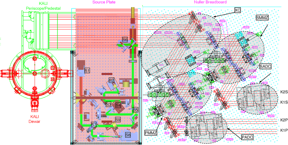
Fig. 13. Schematic of the nuller breadboard (right); the nuller source plate, used for nuller alignment and shear sensing (center); and the nuller camera periscope (top left), which feeds light to the entrance window at the bottom of the nuller dewar (left). The primary and secondary beams from K1 and K2 enter at the lower right of the figure. The shaded areas on the nuller breadboard indicate the locations of the primary and secondary ADCs, the primary and secondary MMZs, and the cross combiner (XC); Fig. 14 provides an expanded view of the nuller breadboard. The output of the nuller source plate is injected toward the nuller breadboard via beamsplitter S6. The nuller source plate includes laser (via collimator S1, arranged vertically, and fiber-fed from a 633 nm laser) and white-light (S2) sources which are combined at beamsplitter (S5). The white-light source path includes a collimator and spatial filter (S3), and a chopper wheel (S4) synchronized to the real-time system. Light returned to the nuller source plate is directed to CCD alignment camera S8 via beamsplitter S7. Element S9 is a Risley prism used during alignment to account for angular dispersion in the nuller breadboard.
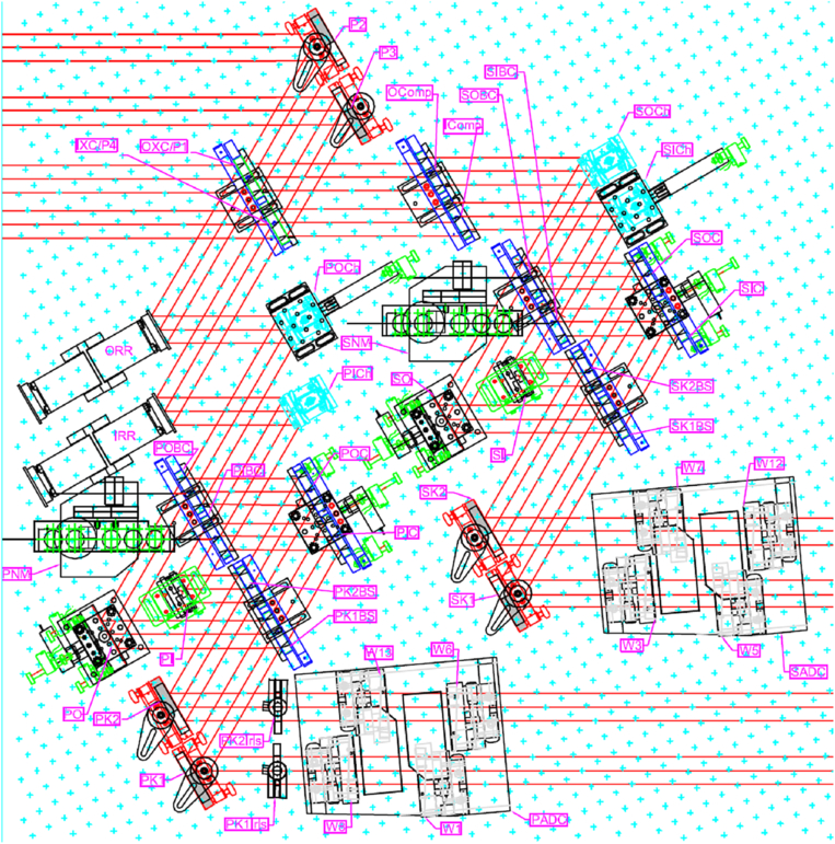
Fig. 14. Expanded view of the nuller breadboard from Fig. 13. Light enters from the lower right. PADC and SADC are the atmospheric dispersion compensators for the primary and secondary beams, implemented with translating ZnSe wedges. Fold mirrors PK1&2 and SK1&2, used for alignment, fold light to the primary and secondary MMZs. The primary MMZ includes two pairs of beamsplitters/compensators (PK1BS & PK2BS and PIBC & POBC), a common fold mirror pair on one side (PIC & POC), and an inner (PI) and outer (PO) fold mirror on the other side; the secondary MMZ is similar. The outer mirrors PO and SO for the two MMZs include PZT actuators for vernier pathlength control. The “dark” outputs of the MMZs are folded into the cross combiner (XC) using angular chopper mirrors POCh, PICh, SOCh, and SICh, which are used during the gated-mode fringe acquisition process; two of these mirrors also include PZT actuators for vernier pathlength control. Fringe-scanning (“rapid ramp”) mirrors ORR and IRR on the primary XC inputs support cross-combiner fringe demodulation. The cross combiner implements a standard Michelson combiner with beamsplitter and compensator IXC and IComp for the combination of the inner outputs of the two MMZs, and similarly with OXC and OComp for the combination of outer MMZ outputs. The four XC outputs exit the breadboard at the upper left and are directed toward the four camera ports via the KALI periscope. Items PNM and SNM are metrology beam launchers which inject into the “bright” outputs of the MMZs as discussed in § 2.11.
2.10.1. Optics: Nuller Breadboard
Light from the two “primary” and the two “secondary” beams enters at the lower right of Figures 13 and 14. Longitudinal atmospheric dispersion compensators (ADCs), consisting of motorized translating wedges of ZnSe, correct for systematic and variable dispersion. The primary and secondary light is then directed into the primary and secondary MMZs. For each MMZ, there is an outer and inner path through the interferometer, and the outer mirrors include PZT (and manual) actuators to allow for vernier path-length adjustment between the two paths. The inner and outer dark outputs of the primary and secondary MMZs are interfered at cross-combiner beamsplitters. Path-length modulators in series with the outputs of the primary MMZ provide a 20 Hz triangular OPD modulation for the cross combiner, and there are additional PZT actuators for vernier pathlength control between the primary and secondary inputs. The four cross-combiner fold mirrors are mounted on fast angular choppers, used during gated-mode fringe acquisition. Also shown are metrology beam launchers injected via the unused bright outputs of the MMZs. These launchers were ultimately not used in operation, as commissioning tests with the launchers showed that cophasing errors attributable to unmonitored paths between the nuller and FATCAT were primarily small drifts that could be accommodated within the (low) bandwidth of the nuller servo.
2.10.2. Optics: Nuller Source Plate
The nuller source place, shown in the center of Figure 13, is used for nuller alignment and calibration. The source plate includes a fiber-fed HeNe boresight laser collimator and a ceramic-element thermal source. The thermal source is collimated, spatially filtered, combined with the laser boresight, and injected back toward the nuller breadboard. The source plate includes a chopper wheel located near the pinhole which is synchronized to the real-time system to allow coherent detection of the white-light source during nuller breadboard alignment. Retroreflected light from slide-in corner cubes either on the nuller source plate (for coalignment of the nuller laser and white-light sources), at the entrance to the nuller breadboard (for coalignment of the nuller camera ports), or in the transport optics (for coalignment of the nuller and FATCAT), is directed to the nuller alignment CCD camera. A Risley prism in series with the boresight laser is used to account for the dispersion in the wedges of the nuller optics so that the laser boresight correctly traces the 10 μm path after exiting the nuller breadboard. Note that the stimulus-injection beamsplitter remains in place during observations, enabling the laser boresight, stopped down in diameter with an iris, to be sensed at the DSM using its shear sensor for real-time beam-train shear adjustment.
The four outputs of the nuller breadboard are directed to the nuller camera via a periscope to a fold mirror beneath the dewar, as shown at the top left Figure 13; the camera is described below.
2.10.3. Camera
The nuller camera, KALI (“Keck Aperture Nulling Interferometer Camera”; Creech-Eakman et al. 2003), uses a large (40 cm × 120 cm) LN2/LHe dewar, accepting four beams through a ZnSe window via a fold mirror beneath the dewar. The dewar includes motorized mechanisms (via ferrofluidic feedthroughs) for aperture, pinhole, filter, and prism sets (along with manual focus mechanisms for the first two lens sets); only the typical settings are given below. The camera internal optical path is illustrated in Figure 15. Light enters through a pupil mask (typically 20 mm diameter) and is focused by a Ge singlet (172 mm focal length) onto a pinhole mask (typically 160 μm diameter) at f/8 with respect to the pupil mask. Note that the geometric beam size at the pupil mask is a 31 mm diameter half-circle. The selection of aperture mask diameter and pinhole size was a compromise between the degree of spatial filtering and the system throughput. Following the pinhole is a Ge singlet recollimator (56 mm focal length), filter (typically a 7.7–13.5 μm bandpass), and prism (typically a “high-resolution” direct-view ZnSe-ZnS pair). The four beams, at this point arranged in a square grid, are multiplexed onto a common pyramidal mirror. While the prior optics are cooled to 77 K, the remaining elements are in a LHe “coldbox”, including a long wave block filter and a final biconvex Ge relay (60 mm focal length) that focuses light onto the array. The clocking of the prisms and the angles of the fold mirrors result in four dispersed spectra, each 3 × 20 pixels (coadded in software to 1 × 10), arranged in a square pattern on the array.
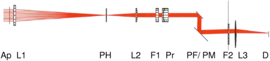
Fig. 15. KALI camera optical path. KALI accepts four beams from the nuller breadboard through a ZnSe window in the bottom of the dewar, and has separate, but co-mounted, beam trains for each beam through the fold mirrors PF, and common elements starting at the pyramid mirror PM. The detector D and final lens L3 are in the cold box, fed through blocking filter F2; the prior optics are maintained at 77 K.
The array is a DRS HF-128 128 × 128 high-flux silicon BIB array with 75 μm pixels, operated at 10 K, slightly above the cold-box temperature, for best sensitivity. Similar to FATCAT, the array is controlled by a combination of commercial front-end electronics (Wallace Instruments) that include clock buffers, bias control, preamps, and 14 bit digitizers, combined with custom electronics for clock-pattern generation and data interface to the real-time system. The 16 digitized camera outputs are multiplexed into four data streams to four camera interface cards in the nuller VME rack; two additional camera cards are used for clock generation and bias control. The 2.5 ms array readout is synchronized with the 20 Hz modulation of the rapid ramp mirrors on the nuller breadboard, which uses five 5 ms ZABCD bins on each of the up and down strokes. Unlike the shorter wavelength arrays, the reads for this array are destructive, and the Z bin data are not used. In operation, the system is mostly background limited, with read-noise contributing about 1/3 of the total variance in the measurement of a broadband fringe quadrature.
2.10.4. Control Aspects
The nuller is phase stabilized at high bandwidth using FATCAT at K band on the two long baselines; details of that system are described in § 2.7. One important aspect of the stabilization is accounting for the effects of atmospheric water vapor. While the dry atmosphere is not very dispersive in the near- and mid-infrared, the water vapor contributions are very dispersive, so that even though water vapor is typically a small contributor to total OPD, the dispersion must be accommodated to allow high accuracy cophasing (Colavita et al. 2004b; Colavita 2010). In practice this means that the K-band system must separately estimate the contributions of dry air and water vapor, and account for them in the feedforward targets generated for the nuller FDLs, which cannot simply be slaved to the K-band FDLs. In addition, a separate feedforward target must also be provided to the nuller ADCs.
The nuller ADCs correct variable atmospheric dispersion, quasistatic dispersion from the basement OPD differences, and residual static dispersion from optical elements in the beam train. Using only group and phase delay measurements, the ADC zero point has a 2π ambiguity; this was calibrated using the spectral phase curvature measured from internal fringe tests. In operation, a quasistatic initial target for the ADC—before enabling the starlight servo—is determined based on the LDL position, the basement temperature and humidity, and a dispersion model, to enable convergence to the proper lobe.23
While the cophasing system controls most mid- and high-frequency phase and group delay errors, the nuller itself, at lower bandwidth, must adjust the FDLs to acquire and track the fringe phase, control the nuller ADCs to minimize group delay, and adjust the three nuller vernier delays between the inner and outer paths of the MMZs and the primary and secondary cross combiner paths so that the fringe quadratures measured at the four outputs of the breadboard can be coherently combined. These control loops are illustrated in Figure 16.
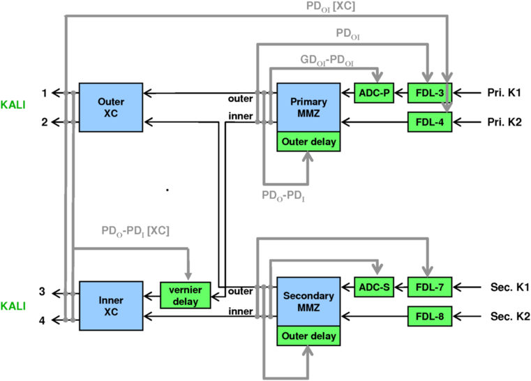
Fig. 16. Nuller control flow in null-peak sum-difference mode as used for data collection. In the figure, PD and GD refer to phase delay and group delay, and the suffixes O, I, and OI refer to data from outer ports only, inner ports only, and the coherent phasor combination of the outer and inner ports. As there is only a single camera shared among the two MMZs and two cross-combiners, the various control loops are active at different times within the micro-sequence. The gated-mode control flow, not shown, is similar.
Because the single nuller camera is shared among the MMZs and the cross combiner, nuller control is time-multiplexed using two different micro-sequences (Colavita et al. 2010b, 2009, 2008, 2006; Booth et al. 2006; Garcia et al. 2006). The gated-mode micro-sequence is used for fringe acquisition, employing conventional fringe scanning implemented by the FDLs and the rapid ramp mirrors on the nuller breadboard to measure the MMZ and cross combiner fringe quadratures. These measurements are used to control the four nuller delay lines as indicated in Figure 16. Differences in the quadratures between the inner and outer paths are used, on bright stars, to adjust the three vernier actuators on the nuller breadboard. Finally, the difference between the group and phase delays is used to control the primary and secondary ADCs. In this gated-mode micro-sequence, the four angular chopper mirrors on the nuller breadboard are used to point away different beams during different sequence phases to allow disentanglement of the observed fringe quadratures.
When the OPDs have converged to less than ∼1 radian, nuller control switches into Null-Peak (NP) mode. In this mode, the angular choppers are disabled, the FDL scanning modulation is replaced by 0 or 180° phase steps, and the FDL and ADC commands are derived from coherent combination of the signals from the four camera ports. NP mode uses a 400 ms long micro-sequence divided into eight 50-ms slots. Two of those slots are used to implement low-bandwidth control on the long baselines; five are used to measure the coherent leakage at null; and the final slot is used to implement low-bandwidth control on the short baseline, and also to measure the coherent leakage at peak (i.e., at anti-null) to serve as an in situ photometric calibration. This is our most sensitive mode—NP mode has a 2 × higher S/N in our application than fringe scanning for control of the FDLs for the MMZs—and all science data are taken in this configuration. The NP mode also has the fundamental advantage of directly servoing on the key observable, the null leakage, rather than indirectly controlling the null leakage by maintaining a particular phase offset.
2.11. Path-Length Control
The KI OPD control system uses a combination of feedback and feedforward control using starlight and other sensors. Fringe measurements from FATCAT are used to provide feedback to their collocated delay lines (typically with a 15 Hz bandwidth, along with selected narrow-band tone suppression), as well as feedforward to the nuller delay lines as discussed in § 2.7 and Colavita et al. (2010a). The non-starlight sensors used for OPD control are described below; see § 4.3for a more detailed performance discussion.
2.11.1. Coude (Ac-Coupled) Metrology
The interferometry basement from the fringe trackers through the FDLs exhibits low levels of vibration: fringe jitter (rms first difference) in double pass from FTS corner cubes in front of the FDLs is typically < 50 nm, and thus is a small contributor to the error budgets. On the other hand, without compensation for the path-length fluctuations from the FDLs to the telescopes, it is not possible to maintain reliable fringe lock, and metrology of that path is required. The solution employed for most interferometer modes was to add metrology, launched from just outside of the starlight clear aperture in front of the FDLs, as shown at the bottom of Figure 7, toward the M14 mirrors, and terminating at the M3 corner cubes in the DSM (Fig. 5). This optical configuration (“coude metrology”) avoided the use of dichroics, and also avoided interference with centered alignment and metrology beams, at the expense of some tilt-to-piston coupling in the sensing. Operationally, PZT fine adjusters on the beam launchers were used to optimize the pointing of this metrology to the DSM corner cubes for each star.
The beam launchers used for this system were identical, except for the beam expander, to those used for monitoring the FDLs described in § 2.6, and were fed from remote source plates in the computer room. The electronics were identical, too, except for the use of APD detectors to provide higher S/N. However, during earlier testing it was discovered that the polarization properties of the individual beam trains led to signal dropouts (with respect to our S/N margins) of this polarization-sensitive metrology system at certain azimuth angles.24 The solution employed was a polarization rotator at the output of the launchers. The launchers output circular polarization, and the rotator just used a quarter-wave plate, converting the polarization back to linear, which tracked the telescope azimuth. With an appropriate zero point for the rotator, this system provided consistent performance at all telescope orientations. As this metrology was used for vibration control only, it was high-pass filtered at ∼1 Hz, so that it wasn’t necessary to worry about its zero point or momentary dropouts, and was used as a feedforward signal to the FDLs via the low-latency path described in § 2.6.
2.11.2. Accelerometer Feedforward
To monitor the rest of the optical path from the DSM corner cubes to the Keck primary, an accelerometer-based feedforward system was implemented. Figure 17 shows the deployment of accelerometers on the system, including six accelerometers, total, symmetrically mounted to three primary mirror segments, and three accelerometers, each, on the secondary and tertiary mirrors. There are also two accelerometers on the AO bench, aligned and adjacent to the input and output beams, and a final accelerometer on the DSM that serves as the tie point to the coude metrology (see also Fig. 5). To within the limitations of the sensors, this system allows correction for rigid-body motions of the three primary telescope optics, AO bench, and DSM, as they project onto the interferometer’s optical path.
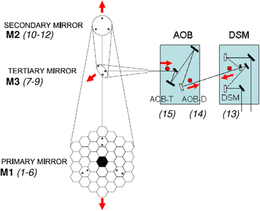
Fig. 17. Accelerometer configuration on the telescope, AO Bench, and the DSM (see also Fig. 5). The arrows represent the orientation of the sensing axes of the accelerometers. The accelerometer measurements are converted to position, filtered, and combined to yield an OPD estimate as 2〈M1〉+2〈M2〉+√2〈M3〉+AOBT - AOBD - DSM.
Quartz-flexure accelerometers were employed, with local, custom gain-strapped preamplifiers to accommodate the long signal runs required to cable the telescopes. The data acquisition systems installed in auxiliary crates in the AO computer rooms on the telescopes’ Nasmyth platforms ran synchronously with the FDLs, triggered at the 4 kHz rate of their fastest loop. The processing steps included simultaneous data acquisition, unit conversion, deconvolution of the antialiasing filter in the preamplifier, double integration from acceleration to position, and high-pass filtering to limit low-frequency noise propagation from the double integration. The high-pass corner frequency of 0.7 Hz was chosen so that the accelerometer position noise spectrum remained below the uncorrected atmospheric OPD power spectrum. Finally, the 15 sensor signals were combined as shown in Figure 17 to yield the feedforward signal used by the delay lines.25 However, in practice, the secondary mirror was usually excluded from the sum, as its mechanical response to focus offloads from the AO system exceeded the dynamic range of the high-gain signal chain.
The achieved end-to-end rejection of the accelerometers in conjunction with the FDLs is 5 × or greater from 7–60 Hz, limited by latency at the high end and the noise-limiting high pass filter at the low end. Between runs, the accelerometer system captures 10 s long, 1 kHz data bursts every 1000 s, useful for long-term trending of the disturbance environment. It’s worth noting that while the coude metrology system remained essential to system operation, the accelerometers played a less critical role over time as the disturbance environment was better controlled, and the fringe tracker was augmented with narrow-band suppression capability: see § 4.3 for a more detailed discussion.
2.11.3. Constant Term (CT) Metrology
Prior to integration and test of the nuller, we were uncertain if the relative optical paths between the fringe tracker and nuller to the K/N splitters in front of the FDLs (after which the K- and N-band beams are common mode) were adequately stable at frequencies above the nuller starlight control bandwidth. While subsequent testing verified that the optical paths were indeed adequately stable without additional control, we discuss the constant-term (CT) metrology system for completeness, as it had implications on the system architecture, and also because it was restored and upgraded for the ASTRA project.
A version of the beam launcher design shown in Figure 9 was used, modified as described in the caption, to launch both s and p polarizations. The beam launcher injection was via a rugate beamsplitter in the FATCAT stimulus as shown in Figure 10. The injected light was split by the FATCAT starlight beamsplitter, and both polarizations were propagated toward the telescopes along each arm. A similar implementation was employed on the nuller, in this case, launching via the unused port (bright output) of the MMZs as shown in Figure 13. For both FATCAT and the nuller, the metrology was injected parallel to, and just below, the geometric starlight beam, but within the system clear aperture, toward corner cubes on the telescope side of the K/N splitters.26 Polarizers in front of the corner cubes selected s for the K1 arms and p for the K2 arms; crosstalk between nuller metrology retroreflected from the corner cubes back to the fringe tracker, and vice versa, was accommodated through the use of different absolute and relative AOM frequencies.
The signal processing for the CT metrology was generally similar to that used elsewhere, although more care was required to maintain adequate S/N. In particular, since both the s and p polarizations propagate, the final S/N is lower than for a conventional launcher for which one polarization remains internal to the launcher, and not attenuated, serving as a local oscillator. Thus, in addition to the use of low noise preamplifiers, a bandpass filter was added to the electronics centered at the heterodyne frequency.27 A consequence of the use of this filter was that the metrology would drop out as its frequency Doppler-shifted out of band as the delay lines slewed between targets. However, this was only an issue for sequencing, as continuity between scans was not important in this application.
The system performed acceptably, although care was required to align the beams to the optical axis to avoid shear-induced signal fluctuations (doubled by the corner cubes) as the delay line tracked,28 and to align the polarization axes to avoid leakage. To minimize beam shear caused by motion of the fast tip/tilt mirrors, KAT was usually operated in split actuation mode (see § 2.9) when the CT metrology was used.
2.11.4. ASTRA Metrology Configuration
For dual-star use, end-to-end metrology—more than just the path monitored above—is required to enable accurate cophasing. In addition, and as was borne out in tests, the metrology needs to be coaxial if it’s to be used at frequencies below 1 Hz. Finally, while there was a deliberate design decision for KI to use HeNe metrology whenever possible, the ASTRA metrology system (Woillez et al. 2012b) incorporated a stabilized infrared Nd:YAG laser in order to provide adequate power to monitor the entire beam train to a corner cube in front of the deformable mirror in the AO system. This metrology system was launched coaxially from the aft switchyard between the tip/tilt mirrors and FATCAT,29 and the CT system described above was now used to monitor the quasistatic path from the beam combiner to the Nd:YAG launcher via a common corner cube on the far side of the ASTRA metrology injection dichroic.
2.12. Real-Time Control System
The operation of KI depends critically on its real-time control system, which has been discussed above in the context of control aspects for various subsystems. A short summary of the overall system is given below. More detail is available in Booth et al. (2006, 2002).
The real-time systems on KI are implemented using 11 VME-based crates, most with multiple MVME5500 or MVME2304 PowerPC processors running VxWorks. The crates control FDLs (2); fringe trackers/nuller (2); angle tracker (1); basement motion control (2); accelerometers (1 for each telescopes); and auxiliary motion control (1 for each telescope). In addition to usual network connectivity, bus expanders with reflective memory are used for low-latency communication from the fringe trackers and nuller to the fast delay lines for closed-loop control. A fiber-based serial link is used between the accelerometer crates and the FDLs for path-length feedforward as described in § 2.11. While much of the hardware is off-the-shelf, including various Industry Pack (IP) modules on carrier cards for I/O, there are a number of custom boards including clock boards for hardware and software synchronization; camera interface and control boards, including pattern generation and data read-back from the array electronics; laser fringe counters for the laser metrology systems; and various signal conditioners, drivers, and other interface and special-purpose hardware. As an example, Figure 18 gives a schematic of the controller for one of the fringe trackers.
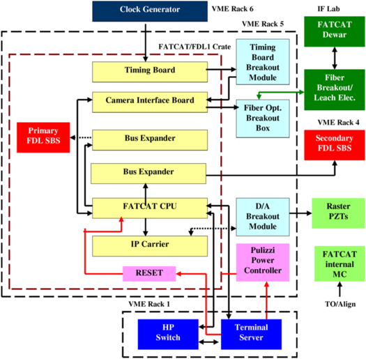
Fig. 18. Schematic of the fringe tracker VME controller. Included in the VME crate are processor cards; a timing card for synchronization among crates connected to the interferometer rubidium oscillator synchronized to the observatory master clock (with coarser timing using NTP); bus expander cards for communication with the delay line crates; a camera interface card for control and data read-back of the fringe-tracker array via a fast fiber link; and I/O modules for driving the raster mirrors for maintaining fringe-tracker alignment. The crate also includes remote reset and power-control functionality.
At the lowest level, all of the real-time systems run VxWorks, although different application programming interfaces (APIs) are used. High-rate applications, i.e., the FDLs and the fringe and angle trackers, use the Real-Time Control (RTC) toolkit (Lockhart 2002) which was developed at JPL. RTC is a toolkit for distributed real-time systems that provides configuration, telemetry, command interface, inter-process communication (IPC) for real-time components, process control, hardware abstractions for sensors and actuators, and device drivers.
Lower-rate applications use the Experimental Physics Industrial Control System (EPICS), which is widely used at Keck Observatory (Lupton 1995), to implement similar functions as needed for KI. The applications include the motion control system that implements the functions needed for aligning and maintaining the beam train, including control of a large number of motors, stages, Picomotors, shutters, and LEDs. While most of these devices are static during operations, the motion control system also controls the active secondary coude train, the KAT DCRs, and the nuller ADCs.
The non-real-time systems run on UNIX workstations, and include user interfaces, observation sequencers, and various RTC services. CORBA (Common Object Request Broker Architecture) is used to provide platform & language independent interfaces to RTC objects. The key RTC services are: (1) the Telemetry Server, which implements a subscribe/publish architecture for each telemetry item, allowing for multiple suppliers and consumers (e.g., graphical user interfaces [GUIs] and archivers); (2) the Archiver, a CORBA client used for recording all of the engineering and science data; and (3) the Configuration Server, which controls access to configuration items maintained in a database repository (PostgreSQL). As an example, Figure 19 illustrates the CORBA interfaces for the fringe tracker. In addition, there is a CORBA/Keyword interface to the Keck Task Library (KTL; Lupton & Conrad 1993) also used at the observatory.
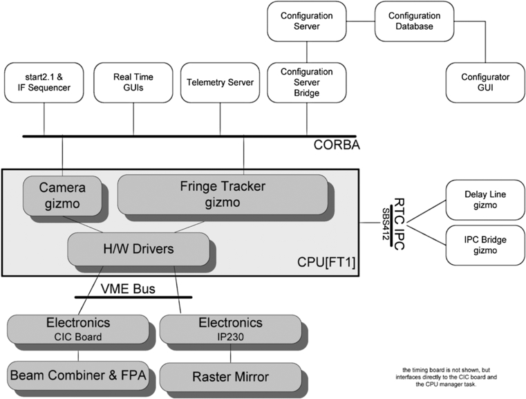
Fig. 19. FATCAT software interfaces. In the RTC taxonomy, FATCAT is an RTC Gizmo—a commandable CORBA object—that incorporates the servo, mode machine, and data; a separate camera gizmo encapsulates the detailed camera control providing, for example, clock-pattern generation and control, control of hardware coadding of subreads, and shared access to the array detector by two fringe trackers using different areas of the chip. RTC hardware drivers are used to access the physical hardware, and an RTC IPC module is used for interprocess communication with the FDL crate for closed-loop control using the bus expander. CORBA services for commanding, configuration, and telemetry, are illustrated at the top. Not shown are the CPU managers that are responsible for booting and managing processes and gizmos on a CPU.
Engineering GUIs for the real-time systems typically use a JAVA framework allowing users to easily configure numeric and graphical telemetry displays, as well as to provide commanding, to suit the application; GUI updates can be made on-the-fly. Engineering GUIs for the non-real-time systems are typically written in Python and IDL, and are used for control and read-back of the various devices for alignment, as well as for system initialization and startup. These include IFOper (quick-look monitoring and control GUI for light sources and motion control devices, including stages, dc motors, Picomotors, PZTs, shutters, targets, & LEDs), IFSys (high-level configuration, health monitoring, and control of various RTC services, utilizing a centralized server application to manage and respond to client GUI commands.), aoOper and aoChop (quick-look monitoring and control GUI for the AO), and hand paddles for the AO field-steering mirrors and M7S mirrors.
The level of observing sequencing required to ensure collection of the proper calibrations, especially for the nulling mode, and to sequence through the various stages to reach the final data-collection state, would not be practical without automation. The observing sequencers, while using different technologies earlier in the project, moved to SMC (State Machine Compiler) to implement the mode machines within the RTC CORBA framework. While the nuller sequencer is monolithic, a hierarchical implementation was used for subsequent (new) sequencers, allowing for implementations incorporating multiple copies of different real-time systems: the most complicated sequencer employs 20 subsequencers.
2.13. Alignment System
Interferometer alignment is typically an involved process because of the number of optical elements involved. At KI, there are additional complications arising from, for example, the dual-beam configuration, the large wavelength range, and the on- and off-axis coude systems. The alignment tools for KI have improved significantly since first light, evolving into a robust system.
While approaches to alignment using fixed stimuli outside of the clear aperture were considered earlier in the project, we ultimately used on-axis stimuli and sensors, and made extensive use of a custom flip-in shutter mechanism for moving shutters, targets, and irises in and out of the beam train at different locations. An outline of the approach used for daily alignments follows.
The coaligned white-light (WL) source and laser boresight from the FATCAT stimulus (Fig. 10) serves as the alignment reference. The system is configured with the FDLs at the back, and the fast tip/tilt mirrors in the center of their range. A stopped-down version of the stimulus is threaded from FATCAT to irises at the input of the fast delay lines by adjustment of the FATCAT dichroics, and onto targets at the M14 mirrors by adjustment of the FDL input folds (see Fig. 7). Alignment corner cubes on a slide-in stage in the aft switchyard (see Fig. 7) are then used to retroreflect the FATCAT boresight and WL source to align FATCAT and KAT, and to set the zero points of the back-end alignment cameras (BCAM). In particular, for FATCAT, the WL source is used to optimize alignment into the single mode fibers, and to adjust the camera internal alignment to locate the spots at the specified pixel locations (using a narrow-band filter in the aft switchyard for repeatable spectral alignment). For KAT, the WL source is used to align the image to the nominal tracker zero point.
When the nuller is used, a similar process is followed using its boresight laser and WL source (Fig. 13), threading it to M14. Nuller alignment corner cubes on a slide-in stage in front the nuller breadboard are then used retroreflect the nuller WL back to the nuller breadboard and camera (see Fig. 7). Using the WL source chopper wheel with the nuller real-time system configured for lock-in mode, the nuller is aligned, and the pointing onto the four pinholes in the camera is optimized. This employs a multistep process that uses the reflection from only one of the four nuller corner cubes at a time, and the correlated flux on a selected camera port to provide feedback to adjust remote-actuated nuller breadboard folds; the process is deterministic, yielding consistent alignments.
Coalignment of the nuller and FATCAT uses the FTS corner cubes in front of the K/N beamsplitters (see Fig. 7), which return both the FATCAT and nuller boresight lasers to the CCD camera on the nuller source plate, allowing adjustment of the N-folds, adjacent to the K/N splitters in Figure 7, to make the spots from the two boresight lasers coincident.
For aligning the LDLs, flip-in LED sources at M11 and M9 (see Fig. 1) are used, which are viewed using BCAM adjusted to a finite conjugate, in conjunction with a sequencer that controls the motors on M11 (M14 is normally not adjusted). Another LED at M8 in the telescope coude crypt is used with BCAM to sense the alignment of M9.
Aligning the coude train uses measurements at different telescope azimuths to adjust the positions of M6 and M7 to provide a stable image and pupil as the telescope rotates. It uses two sets of sensors: (1) flip-in LED sources at M6 in the coude train and M4 in the DSM whose position is measured using BCAM, and (2) flip-in targets illuminated by the stopped-down FATCAT boresight laser whose position is observed with local video cameras. The same approach is used for both the primary and secondary coude trains, with the latter adding offsets to the harmonic model used for pointing the off-axis M6 and M7 tracking mirrors.
Pre-run alignments register the DSM pupil to the AO pupil, and the final daily alignment steps coalign the interferometer and AO boresights. This is achieved via a normally-shuttered corner cube on the AO bench behind the IF dichroic beamsplitter (item 27 in Fig. 4), which when open puts an image of the FATCAT boresight on the AO alignment camera, which can be compared to the location from the AO white-light stimulus (item 22 in Fig. 4). The AO stimulus can also be sensed on the interferometer fringe and angle-tracking cameras to provide another indication of alignment. This stimulus is especially useful for AO optimization to maximize the Strehl on FATCAT, measured via use of the raster mirror on the FATCAT breadboard. The interferometer boresight laser can also be viewed using local video cameras viewing flip-in targets on the DSM, which among other functions provides definitive checking on vignetting in the long beam train.
All of these alignment tasks have automation tools, coded in Python for ease of development and access to a large variety of interferometer components, including Keyword and EPICS-based motion control and sources, Ethernet-based video cameras, and CORBA-based real-time objects and telemetry. The automation greatly reduces the time required for adjustment, as well as minimizing the likelihood of error. In addition, there are alignment sequencers used for (1) night-time LDL moves (which use the position of the interferometer boresight sensed on flip-in targets at M9 and M4 using local video cameras) as pupil and image references; (2) alignment of FATCAT and KAT to the FATCAT boresight returned by local corner cubes; (3) alignment of the nuller using chopping mode on the AO system; and (4) alignment of the beam-train shear using measurements from the shear sensors on the DSMs.
3. Instrument And Science Operations
3.1. Observing Modes
KI supports a number of different observing modes. A list of these modes, their limiting magnitudes, and their summary performance, is given in Table 2. The high sensitivity V2 modes at H, K, and L band provide spectral resolutions from four pixels across the H band (H4) to 42 pixels across the K band (K42). The nulling mode uses a split pupil to implement a four-beam nuller cophased using K-band light, and provides 10 pixels across the N band (N10), in addition to simultaneous K-band V2. The split-pupil V2 modes allow simultaneous measurements at L band and either K or H band. The ASTRA self-phase-referenced (SPR) mode divides the full pupil with a beamsplitter, using part of the light to stabilize the optical path to allow long integration times at higher spectral resolution (330 pixels across the K band; K330) on a second camera. Finally, the ASTRA DFPR mode, demonstrated toward the end of the project, implements dual-field phase referencing on a science target stabilized using an isoplanatic reference star.
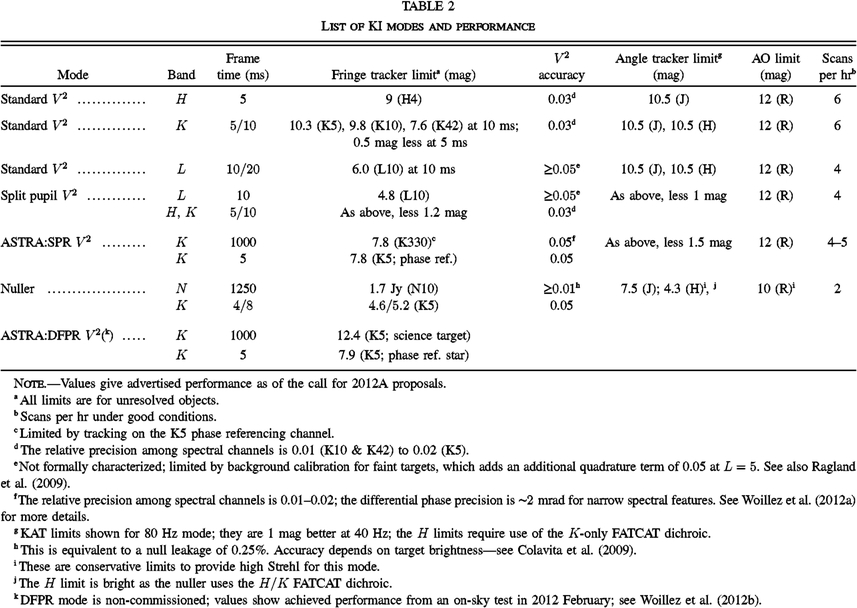 |
3.2. Instrument Operations
3.2.1. Pre-Run Setup
Despite its complexity, KI achieves very high instrument uptime, typically 90%, aided by good practices with respect to configuration control, maintenance, and documentation. KI observations were scheduled into observing campaigns during bright time, and significant instrument alignment and checkout occurs before going on sky. Ideally, all steps to bring the instrument into an operational state would be fully automated, in order to prevent human error and provide repeatability. In practice, a number of manual steps are involved, and a simple, but invaluable, tool is a continually-updated instrument checklist including week-before, day-before, day-of-the-run, and daytime and nighttime activities required to achieve successful operations. The checklist also includes threshold values of quantities such as measured array read noise and FDL tracking jitter, which if exceeded, require additional actions. The use of a rigorous checklist helps guard against more insidious errors where misconfiguration of, say, an OPD feedforward system, could be misconstrued during observations as simply poor seeing. The checklist also includes certain quarterly or biannual actions, such as beam-train collimation checks and FDL tracking jitter tests. In steady state, the effort to operate the interferometer, and maintain the interferometer hardware and software infrastructure as a facility instrument for observers at all levels of interferometry familiarity, was approximately 4 FTEs; it was slightly higher when the nuller mode was routinely used.
The degree of advanced setup leading up to an observing run depends on the mode. For all modes, the DSMs must be reinstalled if they had been previously removed to allow access to AO by other instruments, configured for either single or split pupil mode, and coaligned to AO. The internal beam train must be properly configured, and the various instruments configured. The RTC database includes a number of tagged sets which enable proper configuration of the real-time software; the high-level configuration tool IFSys helps to automate this process to minimize errors. For all modes, internal fringes are tracked to confirm proper operation and the expected delay offsets with respect to the metrology zero points. For the nuller, while the dewar is always maintained at 77 K via an LN2 autofill system, during pre-run setup the camera is manually cooled to LHe, and an extensive alignment and checkout procedure begins. This procedure concludes with a full-up daytime nuller sequence using the nuller’s internal source and the observing sequencer, with the results processed through the nuller data pipeline to confirm proper operation. This procedure is also used to select the four 3 × 20 pixel regions of the array used by the nuller, as well as to determine channel wavelengths using internal fringes. An abbreviated version of the nuller sequence is also used on the first day of the run to manually adjust the nuller vernier stages to be in the center of their PZT actuator ranges.
Routine daytime setup for all modes includes setting the LDL position for the first observation sequence of the night, beam-train alignment, beam combiner and camera alignment, array read-noise calibration, metrology alignment, and coalignment of the various systems; details are given in § 2.13. The final steps of daytime beam-train alignment include telescope azimuth rotations to thread the beam correctly through the telescope coude train to the DSM. Beam-train alignment is facilitated by the alignment sequencers described in § 2.13.
The final pre-observing checkout includes a detailed configuration check, final calibration and coalignment of the various systems, and end-to-end checks including a beam-train vignetting check, and acquisition of the AO stimulus on the angle tracker.
3.2.2. Nighttime Operations
All observing modes employ various sequencers to ensure consistent and efficient data collection as described in § 2.12. In addition to the primary V2 and nuller sequencers, dedicated sequencers are used at different parts of the night, for example, to enable rapid LDL repositions, to adjust the beam-train shear for nuller targets, and to optimize the nuller alignment between clusters, as described in § 2.13.
Several software tools are used to monitor system performance throughout the night. An alarm-handler system is used to monitor the state of the various systems, particularly motion control, that use the EPICS framework. IFSys monitors the health of the RTC components. Finally, the engineering GUIs are configured with threshold values on key telemetry to allow quick-look views of system state and to aid debugging. With respect to the science data quality, quick look analysis of the V2 and nuller data is initiated at the conclusion of each scan to further aid in performance monitoring, as well as to optimize science observations, and if appropriate, to make changes to the scheduled observing program. The top panel of Figure 20 gives an example of phase jitter (rms first-difference of fringe-tracker phase) versus time—one of the most useful metrics for assessing instrument stability and performance. High levels of jitter cause both a reduction in fringe visibility, and at higher levels, prevent reliable phase unwrapping in the fringe tracker. The plot shown is representative in exhibiting an instrumental noise floor, a slight dependence on target magnitude, and a slow variation over time attributable to changing atmospheric seeing.
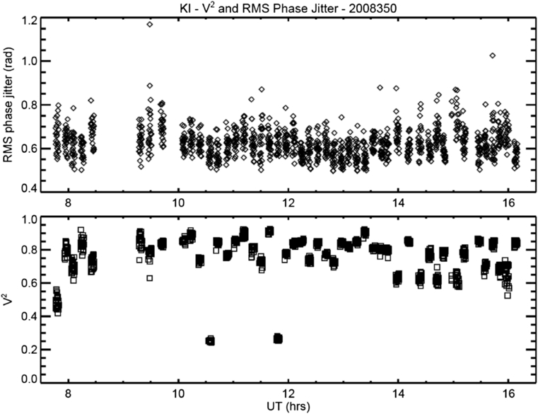
Fig. 20. Wideband incoherent V2 (bottom panel) and rms phase jitter (top panel) for various targets during a night of K-band V2 observations.
3.2.3. Sample Observing Sequences
Figure 21 illustrates a typical V2 observing sequence, emphasizing the parallelism of the various parts of the process. As noted previously, KI does not include separate photometric channels, and we instead rely on the fact that if intensity fluctuations are uncorrelated between apertures, knowledge of the average fluxes of the individual apertures over the data-collection interval is adequate for full correction of the data (Shaklan et al. 1992). At PTI, only a single ratio measurement of the separate fluxes was taken at the end of a scan, and primarily served as a diagnostic, as application of the ratio correction was not shown to improve the data quality. However, at KI the observed intensity fluctuations are larger, and in particular, display a pink noise power spectrum. Subject to these statistics, interleaving the ratio measurements as shown in Figure 21 provides a more accurate measure of the average flux over the interval, and the ratio correction computed from these five sets of 5 s single-aperture fluxes generally improves the data quality of the 125 s of fringe data. The V2 sequence also includes a single dark measurement at the end, implemented with a shutter. While this approach is adequate for photometric calibration of H/K data, for L-band observations, an additional telescope nodding step is required to get a useful dark measurement for calibration (Ragland et al. 2009).
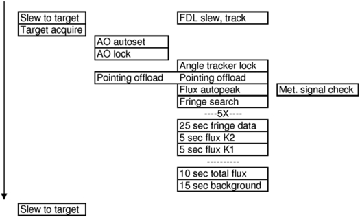
Fig. 21. V2 observing sequencing, illustrating the parallelism of the various tasks.
One other aspect of the sequence is worth noting: the flux auto-peak step prior to data collection (which happens in parallel with optimization of the alignment of the coude metrology). This step uses the raster mirrors on the FATCAT breadboard (Fig. 10) to determine the pointing offset which maximizes coupling into the single-mode fibers. In V2 mode, an offset to the KAT zero-point is used to apply the pointing correction. In nulling mode, where KAT controls pointing to both the nuller and FATCAT, the raster mirror zero points are changed in order to not affect the nuller pointing.
The V2 sequence is very efficient, and for H- and K-band targets, when the seeing is average or better, six or more stars per hour can be observed, as illustrated in Figure 20.
Finally, for the case of the nuller, Figure 22 illustrates the sequencing involved in getting to the point of collecting science data. The first three minutes includes the time for telescope slew, AO acquisition, and acquisition of the four beams on KAT. After a shear adjustment, K-band fringes are acquired, phase referencing is enabled, and background calibrations are acquired on the nuller in gated and NP mode. The next three minutes are spent acquiring and stabilizing nuller fringes using the low bandwidth nuller control system in gated mode. At eight minutes into the sequence, the nuller switches to the NP micro-sequence for data collection, enables the vernier control loops, and after settling, begins science data collection, typically for 12 minutes, for a cadence of about 25 minutes per scan. Addition information on the nuller science sequencing is in Colavita et al. (2009).
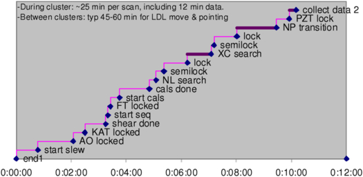
Fig. 22. Observing timeline in nulling mode from the end of data collection on one target to the start of data collection on a second target, including the time required for telescope slew, shear adjustment, acquisition, and settling of the various active systems, calibrations, and the transition through gated mode to NP mode. For targets in the same part of the sky, it takes 10 to 12 minutes from the end of data collection on one star to the start of data collection on the next star.
3.3. Science Operations
3.3.1. Operations Model
All KI science observations were executed in service observing mode. Science observing was performed by staff at WMKO with support from NExScI. Interferometer runs were generally scheduled to take place two to four times during a six month semester, and science and engineering observing both took place during a given run. PI’s and Co-I’s could participate in the observing either from the interferometer observing room at WMKO headquarters in Waimea, or remotely. Remote participation was either data monitoring only, from any computer via a password-protected website showing the near-real-time data reduction, or monitoring of all telescope parameters at one of the Keck Remote Operations sites. Each project was assigned a NExScI contact scientist to help with observation planning and data analysis.
3.3.2. Observation Planning
KI schedule files used a pre-defined ASCII format to describe the sources to be observed along with their properties. The interferometer files were read by the KI real-time software and also translated into the format used by the telescopes. These files could be produced by hand, but generally the getCal program was used.
getCal30 is an interferometric observation planning software suite. Its tools can be used to resolve common star names into standard catalog designations and astrometry; extract visibility calibrators from the Hipparcos catalog according to a variety of geometric, brightness, and astrophysical criteria; compute target zenith and delay accessibility; and interface with the Simbad astronomical database, the PTI and KI sequencer GUIs, visibility calibration codes, and sky visualization software. It can be installed locally on the user’s computer or used via a web interface (gcWeb).
To further assist with investigation planning, the KI observables can be simulated using the Visibility Modeling Tool, VMT.31 VMT allows the user to specify an observation configuration (object coordinates, time coverage), instrument configuration (V2 or nulling mode, spectral band, and dispersion), and a model of the object to be observed that can be specified either as a combination of elementary geometrical morphologies (with user-specified relative fluxes and sky offsets) or as an uploaded FITS image. VMT then computes and plots the resulting KI observables, and is therefore a valuable tool in assessing the viability of a given investigation.
3.3.3. Data Reduction Pipeline
3.3.3.1. Visibility Data
There are two stages of the KI visibility data reduction pipeline. The first stage takes the raw data packets as recorded by the real-time software and applies all instrument calibrations. This software is called Kvis and is run automatically as part of the end-of-night processing. The output of Kvis is several ASCII files which are available to users in the data archive.32
The KI visibility measurement technique and calibration are based on the design implemented at PTI and described in Colavita (1999). Briefly, Kvis combines the individual reads into longer frames (typically 0.1 s) and blocks (typically 5 s). During a single frame the spectrometer phases are referenced to the average wide-band phase and both the coherent and incoherent visibility estimators are calculated with corrections for the zero-point, read noise, wavelength, and photon- and detector-noise biases (using the extended expression in Colavita et al. (2010a; see also Perrin & Ridgway 2005). The balance between the two arms, used to compute the ratio correction, is also calculated at this time, and applied later if selected. During a block, the squared visibility (V2) is calculated coherently and incoherently for the wide-band channel, a weighted average of the spectrometer channels, and individually for each spectrometer channel. The block data are written into the Kvis output files and contain calculated values for the wide-band channel and for each spectrometer pixel. Typically the incoherent values were used for data analyses.
The next processing step is to produce calibrated visibilities, which can then be used for scientific interpretation. The visibility that KI measures on an astronomical object (Vm) is the product of the true object (Vt) visibility and the system visibility (Vs), which accounts for the loss of coherence due to instrumental and atmospheric factors. The system visibility can be estimated using observations of unresolved stars, or stars of known size. In general the system visibility is a slowly-varying quantity, and depends such factors as seeing, alignment, object location in the sky (e.g., dependence of seeing on zenith angle) and the instrument configuration (e.g., integration time).
For visibility data, there are two packages which find and apply the system calibration, wbCalib and nbCalib,33 which work on the wide-band and spectrometer data, respectively. Both of these packages are run by the user rather than automatically as part of the pipeline. In addition to the data files, the user must provide a file listing the source names and the calibrator names, angular sizes and uncertainties. This ASCII file can be produced by hand or by using the getCal program. The wb/nbCalib packages have many options which control which calibrators are selected, how they are weighted and what other corrections to apply, including the ratio correction described above.
An important additional correction, applied to visibility data from the primary fringe tracker camera, accounts for flux-dependent array errors as discussed in Appendix
In addition, the pipeline also produces a differential phase spectrum, referenced to the broadband white light phase. Broad features in the differential phase (slopes or curvatures across the bandpass) are dominated by instrumental and atmospheric effects, and are not likely to contain astrophysical information. However, narrow spectral features can be astrophysically meaningful, as exemplified in, e.g., Pott et al. (2010).
3.3.3.2. Nulling Data
The nuller data reduction is discussed in detail in Colavita et al. (2009). To first order, the null leakage is just the ratio of the fringe amplitude on the short baseline with both long baseline nullers at null, to the fringe amplitude with them at peak. In practice, additional steps are required: In particular, proper data gating is important to achieve consistent performance, e.g., to ensure that all systems are in the proper state and that all servos have settled. This is done objectively, with a set of criteria for system state and servo residuals that is applied consistently to all observations. As for V2 observing, nuller observing interleaves measurements of calibrator stars to measure the system leakage. While not used to date for astrophysical investigations, a differential phase quantity can be constructed from the real and imaginary parts of the null-null phasor. These phases would be subject to the same caveats as for K-band data regarding the interpretation of broad spectral features, and further investigation would be needed to bound the effects of systematic errors in the null leakage.
3.3.4. Archive and Archive Operations
The KI raw data were processed automatically at WMKO immediately following each observing night. Following successful processing the resulting data files were automatically sent to and ingested in an archive located at NExScI. All the KI data are now public and available to users via the Keck Observatory Archive (KOA).35
4. System Performance
4.1. System Throughput
Table 2 includes the advertised sensitivity for the various KI modes from the instrument call for semester 2012A (2012 February–July). These values tie to a throughput budget validated using on-sky data.
From an analysis of 11 nights of K-band data in standard V2 mode between 2008 and 2012, the median “throughput,” from total light in to total detected photons summed over the WL and Spec channels (i.e., both beamsplitter outputs) through the single-mode fibers is ∼250 ph/ms at K = 10. Table 3 presents a summary K-band throughput budget, which shows an effective value of 1.1% from light in to detected photons, consistent with this value. Because we only measure light after spatial filtering by the single-mode fibers, we can’t unambiguously separate Strehl terms from pure throughput terms. However, the error budget includes measured or known values where possible, and the total throughput is consistent with the on-sky behavior.
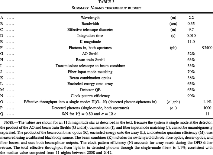 |
For the Strehl terms, we adopt 52% for the AO system, a typical value36 at R = 11. We adopt 63% for the beam-train Strehl, including both static and variable contributions, and adopt 70% for fiber mode matching as discussed in § 2.7. For the clock-pattern efficiency, i.e., the fractional integration time per frame after accounting for array reset and dither retrace, we adopt 90%, appropriate for a 10 ms clock pattern.
The beam combiner, including the product of the external (warm) and internal (cold) optics, the encircled energy onto the array, and the detector quantum efficiency, was measured using a calibrated blackbody source at 16%, total, excluding the input mode match. We allocate this among the three terms, based on other data, as 38% optics, 65% encircled energy onto the active pixels of the array, and 65% detector quantum efficiency. The optics terms, illustrated in Figures 10 and 11, include a 90%-reflective input dichroic, 7 reflective elements (including dielectrics), 5 transmissive elements (compensator, fiber, lens, filter, and prism), and also include apodization by the finite-diameter collimator lens in the dewar. Throughput for the L-band beam combiner is lower, but as that system remained formally shared-risk, we did only limited work to reconcile its performance with the K-band systems.
The 33% transmission to the beam combiner is not a direct measurement, but rather a derived value based on the measured end-to-end throughput and the measurements or adopted values of the other contributors as described above. Starting from the telescope primary, and including the AO system, there are 26 metallic mirror reflections, two hot mirrors (87% total reflectivity from their spectrophotometer scans), and one window prior to the switchyard dichroic. The adopted value corresponds to an effective value of 96.5% per surface, which is plausible, as it includes optics that have been in use for an extended time, including those more exposed to contamination in the coude train (M5-M8) and on the telescope (primary, secondary, and tertiary).
As shown in Table 3, for a K = 11 target the total number of detected photons in 10 ms from both sides of the beamsplitter through the single-mode fibers is ∼1000 for the observed median system throughput. The theoretical S/N for the fringe tracker is given by the usual expression (see Colavita et al. 1999)
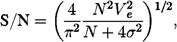
for total flux N, fringe visibility Ve, and read noise σ. In the K5 configuration, a typical value of the read noise for the sum of the WL and five spectral channels used for tracking is 12 e-. We adopt  , slightly lower than a typical value for the system visibility, because the real-time S/N estimator uses a longer effective frame time, and thus suffers more visibility loss than the standard quadrature estimator (see Colavita et al. 2010a). These values give a good match to the S/N reported by the real-time system. Using these values, for 1000 total photons, the corresponding S/N is 11.
KI tracks reliability down to an S/N of 8–10, so from the throughput budget in Table 3, the fringe tracking limiting magnitude at 10 ms is slightly greater than 11.0. It’s worth noting that in principle, in an ideal vibration- and scintillation-free environment, operation down to an S/N of ∼3 would be possible (below which the Gaussian approximation to the noise in the arctangent phase estimator fails). In practice, the environment is never ideal, and a higher S/N is required. In advertising performance for the instrument call, we typically assumed an S/N of 10, and applied 2 × margin to account for non-ideal atmospheric conditions and instrument alignment in order to ensure successful execution of the science program. Thus our advertised performance in the final call for proposals was a magnitude of 10.3 in this mode. A similar set of calculations was done for the other modes.
4.2. System Validation: V2 and Nulling Performance
Both the V2 and nulling modes went through a performance validation process at completion of their development phases. In both cases, spectroscopic binaries were used to provide targets with known fringe visibility or target leakage. More details on V2 validation for its commissioning in 2004 are in Wizinowich et al. (2004); an example observation is shown in Figure 23. At that time, the operational requirements were V2 accuracy of 0.05 to 9th magnitude in K band. Performance improved over time in both V2 accuracy and sensitivity, and the most recent values are incorporated in Table 2, including performance for additional modes and capabilities.
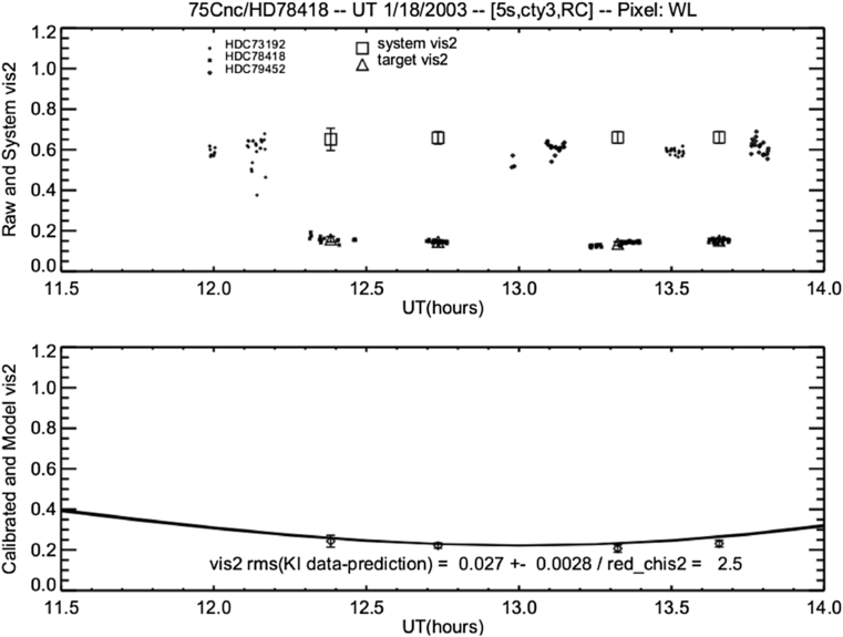
Fig. 23. V2 data vs. prediction from one of the V2 validation tests.
For our most sensitive V2 mode, we achieve a (calibrated) V2 accuracy of 0.03 down to K = 10.3, with a typical cadence of 6 stars per hr; the relative precision among adjacent channels is 0.01–0.02, depending on resolution. In the high resolution ASTRA SPR mode, the V2 accuracy is 0.05, with relative precision of 0.01–0.02, and differential phase precision of ∼2 mrad for narrow spectral features; see Woillez et al. (2012a) for more details. While not formally characterized, L-band V2 accuracy is estimated as 0.05, although it degrades for fainter objects attributable to uncertainty in the background calibration. The split-pupil modes have the same accuracy as the full-pupil modes, but with brighter limits.
The nuller validation process in preparation for beginning its key science program in 2008, and the assessment of its formal performance limits, is discussed in detail in Colavita et al. (2009),37 and also summarized in Table 2. The calibrated null leakage accuracy for bright targets is 0.25%, equivalent to a V2 accuracy of 0.01. Measurements are possible down to 1.7 Jy for compact objects so long as the K-band brightness is sufficient, although the measurement accuracy degrades attributable to systematic terms.
4.3. Vibration Control Summary
As noted in § 2.1.3, vibrations were a problem at first light, and significant effort was expended to deal with them. A trade exists among passive attenuation or isolation of the vibration source(s), passive attenuation of the specific response of an impacted optic(s) through stiffening or damping, and active attenuation at the system level. At KI for risk reduction and robustness of the resulting solution, passive and active approaches were pursued in parallel. While a challenge for the passive approach is to identify which machines or which mounts to address, and there is more discussion on this topic in Hess et al. (2003), passive approaches in general reduce requirements on the active systems, and provide a more predictable vibration environment. While active systems in principle provide an end-to-end solution, not all vibrations are fully observable with high-bandwidth (non-starlight) sensors.
The major mitigation activities were carried out through 2002 September, isolating the largest contributors, and integrating the active systems. The vibration environment continued to improve over time as additional machines were isolated, machines were replaced with quieter (and more energy efficient) units with particular attention paid to their mounting and isolation, and the active systems were optimized in preparation for nulling. Below, we illustrate the vibration environment toward the end of the project with respect to OPD, tilt, and intensity, and illustrate the relative contributions of the different active systems.
Figure 24 shows the contribution to the windowed OPD residual38 of the each of the three active OPD control systems (coude metrology [§ 2.11.1]; accelerometer feedforward [§ 2.11.2], and FATCAT feedback and narrow-band tone suppression [§. 2.11]) on a data segment on night 2010057. The net effect of the three systems is a 2.7 × reduction the rms windowed OPD. The end-to-end coude metrology provides the largest reduction, 1.6 ×, attenuating a number of tonal disturbances between 10 and 100 Hz. The accelerometer feedforward system provides an additional reduction of 1.25 ×, mostly through attenuation of lateral translations of the DSM, AO bench, and tertiary mirror over the range 10–15 Hz. The fringe tracker provides a total of 1.4 × additional rejection, of which 1.15 × is from the ordinary low frequency servo rejection below its 16 Hz bandwidth, and 1.2× is from narrow-band rejection near 24, 29.5, 35, 55, and 59 Hz. Different nights show different detailed behavior, particularly in the tonal contributions, but the figure is representative with respect to the relative contributions of the three active systems for the system configuration and vibration environment at the end of the project. The figure is also qualitatively representative of the relative contributions of the three systems for OPD control for nulling, as discussed in Colavita et al. (2010a).
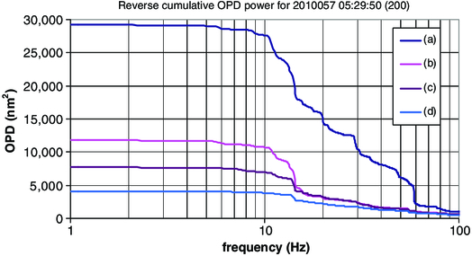
Fig. 24. Reverse cumulative power of the OPD residuals filtered by the V2 window function for night 2010057 near UT 05:30. The four traces illustrate: (a) the uncontrolled OPD; (b) the residual after coude metrology feedforward; (c) the residual after also including accelerometer feedforward; and (d) the residual after also including the fringe-tracker closed-loop servo and narrow-band tone suppression. With all three systems, the windowed residual [square root of the low frequency asymptote of (d)] is 63 nm rms (0.18 rad rms at K band) for this 5 ms window, reduced from 171 nm rms without compensation.
Figure 25 is a power spectrum of the angle-tracker residuals for this for this same segment of nighttime data. KAT typically runs with a ∼3 Hz bandwidth, which is adequate to suppress residual basement seeing. The residuals shown are largely tonal, with a typical rms of 4 mas referred to the sky. Notable, and reflective of the passive mitigation activities, the ∼29.5 Hz tonal contribution attributable to induction motors which used to be a significant contributor, is no longer dominant, and as discussed in § 2.9.2., we deprecated the use of an active control notch to suppress its effect.
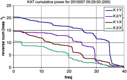
Fig. 25. Reverse cumulative power of the angle-tracker residuals for 2010057 near UT 05:30. An approximate correction for sensor noise has been applied. For these data, KAT ran at 80 Hz, and the rms referred to sky from the square root of the cumulative power is 3–4.5 mas.
Figure 26 is a power spectrum of the normalized total flux,  , for this same segment of nighttime data. The figure is representative of system behavior, in particular, showing a tonal contribution above 10 Hz, and a ∼1/f low-frequency noise spectrum down to the 0.06 Hz limit of the plot. For this night, the rms attributable to the tonal terms above 10 Hz is 0.18, with total rms of 0.22 for f > 0.06 Hz. Three particular aspects of KI’s operation are responsive to this behavior: (1) interleaved (rather than one-per-scan; see § 3.2.3) single-aperture flux measurements, to better estimate the flux mismatch in the presence of the low frequency spectral terms; (2) per-star pointing optimization (the raster process in § 3.2.3), as the coupled-flux PSD gets markedly worse when the fiber couplers are misaligned; and (3) robust fringe finding algorithms, to reject spurious “fringes” attributable to scintillation from the tonal terms (see Colavita et al. 2010a). Additional mitigations between system first light and V2 mode commissioning that improved the coupled flux to its current acceptable state include basement seeing improvements (e.g., insulation of the coude tubes),39 fiber coupler optimization, higher KAT bandwidths through the addition of its fast tip/tilt mirrors, stiffening and damping of the angular modes of various feed optics, and additional source isolation.
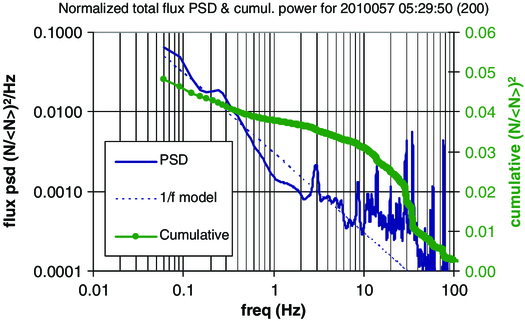
Fig. 26. Power spectrum and reverse cumulative power of the coupled flux for night 2010057 near UT 05:30. The PSD is computed for the sum of fluxes from K1 and K2 on the WL channel normalized by their interval mean. The rms for f > 0.06 Hz from the square root of the cumulative power is 0.22.
4.4. KI Science Output
Starting with first light in 2001, KI was scheduled for more than 250 nights of engineering and science observations. Most science observations arose from successful proposals to the time allocation committees (TACs) overseeing science use of the Keck telescopes, and from the 32 night Nuller Key Science Project conducted by three teams selected in a dedicated NASA-time proposal call. Table 4 gives a brief summary of major KI science topics during the operation of KI, including the number of science observing nights and the number of peer-reviewed papers to-date. A broad overview of KI science is given by Ragland et al. (2012).
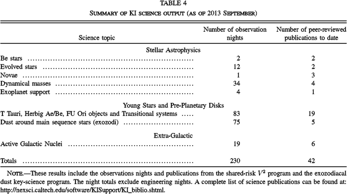 |
The Keck Interferometer was funded by the National Aeronautics and Space Administration (NASA). Observations presented here were obtained at the W. M. Keck Observatory, which is operated as a scientific partnership among the California Institute of Technology, the University of California, and NASA. The Observatory was made possible by the generous financial support of the W. M. Keck Foundation. The ASTRA upgrade to KI was funded by the National Science Foundation under Grant No. AST0619965. Part of this work was performed at the Jet Propulsion Laboratory, California Institute of Technology, and at the NASA Exoplanet Science Institute, California Institute of Technology, under contract with NASA. Thanks to the referee for helpful comments.
Appendix A:: Calibration of Errors from Flux-Dependent Array Errors
Visibility measurements with the primary H/K camera on KI need to be corrected for errors from apparent array reciprocity failure. Reciprocity failure in an infrared array refers to a flux-dependent photometric nonlinearity (Bolin, Linder, & Riess 2005; Schubnell et al. 2010; Biesiadzinski et al. 2011), typically characterized by an error with a logarithmic dependence on flux over a large flux range. The effect is separate from ordinary saturation nonlinearities that occur as the flux approaches the full well of the array, and which are absent at low to moderate flux levels. For KI, the manifestation is a flux-dependence to the measured V2. We approach this phenomenologically—physical mechanisms and behavior in other arrays are discussed in the references—as our primary objective is to improve the data quality.
The results of an internal fringe test are shown in Figure 27 for the primary H/K camera taken in a standard K-band V2 configuration. There is a clear flux-dependent bias to the measured V2, which is, empirically, much larger for the spectrometer data than for the broadband (WL) data, and which is present even at 10-3 of full well. The bias is well fit by a simple logarithmic model. Similar behavior is observed for other configurations of this camera, including different integration times, higher spectral resolutions, different read clocks, and H band versus K band.
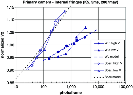
Fig. 27. Flux-dependent V2 biases observed in internal testing on the primary H/K camera. The abscissa is flux per frame in photons. The three traces on the right of the graph are for the broadband WL channel. The circles are for normalized V2 for high intrinsic V2 (∼0.9, normalized to near unity in the graph) and the triangles are for low intrinsic V2 (∼0.1, accomplished via flux imbalance, similarly normalized to near unity in the graph), and for the model described in the text. The three traces on the left of the chart show similar data for a spectrometer pixel, which exhibits a larger effect. The configuration for this test was the primary fringe tracker camera, K band, 5 ms frame time, and a 5-pixel spectrometer resolution.
To account for this effect, a correction is applied to the measured V2 during post processing. The model used is

where N is the number of photons per frame and n0 = 80 photons. The leading coefficient is kWL = 0.063 for the white light channel and kSpec = 0.16 for the spectrometer, i.e., 6.3% and 16% per decade. These parameters provide a good match to most camera configurations. The low-V2 data don’t fit this model quite as well as the higher V2 data, but the data quality are still improved by applying this correction. Figure 28 shows a confirmation of the effect on sky, which yields a best-fit value of kSpec - kWL of 0.11, close to the difference of the values above.
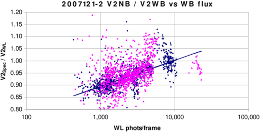
Fig. 28. Measured ratio of the spectrometer V2 to the WL V2 vs. flux from nights 2007121 and 2007122 with the primary fringe tracker at K band, K5, 5 ms frame time, and a 5-pixel spectrometer resolution. The best fit slope (using the Median Absolute Deviation [MAD] metric to reject outliers) gives a logarithmic coefficient of 0.11, which is close to the difference, 0.10, of our adopted correction spectrometer and WL calibration coefficients.
It is notable that the ASTRA H/K fringe tracker camera, which uses the same model of HgCdTe array as the primary camera, while not free of nonlinearities, does not exhibit a strong effect at moderate flux levels. The results of an internal test, similar to that used on the primary camera, are shown in Figure 29, and on the basis of these results, we do not apply any correction to data taken with this camera (We also don’t use the correction for the L-band camera, although it has not been as thoroughly characterized.) As the electronics and optics for this second H/K camera are nominally identical to the first camera, it seems likely that the effect we observe is array-dependent. This variability in the magnitude of the effect among different samples of the same device has been seen by other researchers (Schubnell et al. 2010).
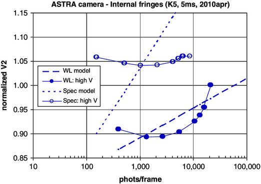
Fig. 29. Flux-dependent V2 biases observed in internal testing on the ASTRA camera. Analogous to Fig. 27, the two traces on the lower right of the graph are for the broadband WL channel, while the two traces on the upper left of the graph are for a spectrometer pixel. Only high intrinsic V2 data were collected for this test. The model traces are the same as for Fig. 27, using the parameters in the text. The logarithmic behavior seen on the primary camera in Fig. 27 is largely absent at moderate fluxes. There may be the onset of ordinary saturation nonlinearity at fluxes >10 k photons/frame on the broadband channel, although this would be at a lower level that expected based on measurements of the primary camera, and thus may represent a different nonlinear effect. The configuration for this test was the ASTRA fringe tracker camera, K band, 5 ms frame time, and a 5-pixel spectrometer resolution.
Finally, it’s worth noting that with good experiment design to match the fluxes of science and calibrator stars, the array behavior shown here largely calibrates out, without the need for the correction. However, regression tests on the 2004 validation data (see § 4.2) show improved performance with this correction, and we adopt the correction for all data taken with the primary H/K camera.
Footnotes
- 4
A list of peer-reviewed science papers is available at http://nexsci.caltech.edu/software/KISupport/KI_biblio.shtml.
- 5
The PIs of the three exozodi key-science teams were P. M. Hinz, M. J. Kuchner, and E. Serabyn.
- 6
When originally designed, KI had additional modes supporting direct and indirect exoplanet detection and supporting observations as described in the early system papers. One of these modes was differential phase (DP; Akeson & Swain 1999), which, using the two Kecks, would employ multi-color fringe measurements from 1.5–4.2 μm to detect the presence of warm, close-in stellar companions. After some development (see Vasisht & Colavita 2004), the DP mode was descoped in 2005, although the camera developed for the DP mode was later deployed for L-band V2. The other modes were to use four 1.8 m telescopes deployed at the periphery of the Keck site. They were to provide additional baselines for synthetic aperture imaging, both as a stand-alone array and combined with the two Kecks, with baseline lengths from 30 to 135 m. In addition, the 1.8 m telescopes were also to be used to implement long baseline narrow-angle astrometry (Shao & Colavita 1992) for indirect exoplanet detection on orthogonal ∼100 m baselines. While the telescopes were designed and built (see Bell et al. 2004), and the necessary permits obtained, this mode was cancelled in 2006, and the telescopes ultimately repurposed for use elsewhere in the US astronomy community. Note that the capability for combining up to six apertures informed some of the details of KI’s implementation.
- 7
The PIs of the four V2 shared-risk teams were W. C. Danchi, S. R. Kulkarni, J. D. Monnier, and W. A. Traub.
- 8
The aperture diffraction limit is 45 mas (λ/D) at K band for the full 10 m aperture. The on-sky beam is slightly larger, ∼65 mas FWHM, attributable to convolution by the Gaussian mode shape of the single-mode fiber. For the nuller, including the effects of the pinhole in the camera, diffraction in beam propagation, and the diffraction pattern of the semi-circular subapertures, the on-sky beam has a FWHM of ∼500 × 440 mas (Colavita et al. 2009).
- 9
For nulling mode, because of residual fixed OPD differences between primary and secondary, the primary and secondary delay line targets are offset by 2 m, and so the effective range is 13 m.
- 10
See § 2.2 for details on the pupil shape. Beam diameters throughout are with respect to the 10 m effective diameter.
- 11
The beam compressors are simple two-mirror afocal collimators, and for large pupil distances, the propagation distances in the 31 mm space are multiplied by the square of 4∶1 compression ratio when translated to effective distances in the 124 mm space.
- 12
The baseline coordinates are E: 51.7023 m, N: 67.4556 m, and Up: -0.0037 m. The typical offset for V2 mode with respect to the metrology zero point is C = 41.043 m.
- 13
An absolute laser distance gauge with mm accuracy, measuring along the length of the LDL track, is also used to confirm each cart’s position.
- 14
For internal testing, the LDL can also be used as a retro-flat by reflecting the beam back toward M10.
- 15
The numbering discontinuity arises because the original design of the LDL system had an option for longer delays by injecting light from M10 to the lower mirror position of the LDL cart in Fig. 6, which would reflect to a fixed mirror mounted to the wall above the exit of the K2 coude tube, and then back to the top mirror of the LDL cart, to be directed to M14.
- 16
The AGC stage also provides a signal-strength indicator useful for metrology alignment.
- 17
One other aspect of this approach is that, due to minor differences in the mode matching of the two fibers attributable to, say, coupler misalignment, the measured phases on the two beamsplitter sides will not be identical if the input Strehl is not `unity. In practice, as long as the couplers were reasonably well aligned, this had no significant operational consequences.
- 18
The threshold is implemented as
 for scalar S/N threshold S0, minimum visibility V0, and measured average flux 〈N〉 and measured read noise σ.
- 19
Typical spectrometer wavelengths for each pixel: 3.47, 3.53, 3.61, 3.68, 3.74, 3.85, 3.93, 3.99, 4.04, and 4.09 um.
- 20
KAT runs internally at twice this rate to implement a CDS readout. Rates slower than 80 Hz are more efficient, as there is less clock overhead attributable to slewing between readout boxes, and more time is available for subreads to improve noise performance.
- 21
During nuller validation, real-time monitoring of the nuller fast tip/tilt mirror tilts using custom laser autocollimators was implemented to confirm that the open-loop tracking of these mirrors was adequate to meet the nuller error budget requirements.
- 22
The division between the two halves is perpendicular to the telescope’s elevation axis. In nulling mode, the AO system image rotator operates in fixed-pupil mode at a 90° setting so that pupil remains fixed at the DSM, with the division vertical, enabling straightforward implementation of the pupil split (see § 2.3). Once split, the separate pupils do rotate with telescope azimuth as the beams are propagated to the interferometry basement.
- 23
Each ADC includes an optical encoder to measure its position. The encoder position is used to generate a compensating target to the corresponding FDL to correct for the ADC’s phase effects, allowing for decoupled group delay and phase delay control.
- 24
Here we are talking about the properties of individual beamlines; for high contrast starlight fringes, it’s the matching of the (imperfect) polarization properties that’s more important (and in addition, polarization effects from oblique reflections are reduced at the longer science wavelengths). Some beam-train symmetry measurements at KI are discussed by Hrynevych et al. (2006).
- 25
Because of limitations in the word size of the dedicated link between the FDL and the accelerometer system, the signal was high-pass filtered before transmission, and restored on the FDL side; the effect was to primarily transmit differences between samples to reduce dynamic range.
- 26
These corner cubes were located just below the geometric starlight beam, adjacent to the primary and secondary FTS corner-cube stages shown in Fig. 7.
- 27
In addition, for the two metrology gauges operating at a 4 MHz offset to avoid crosstalk, as noted above, a digital mixer was used to translate the signal to 2 MHz to employ the standard fringe counting electronics.
- 28
Of course we could have used retro flats instead, trading tilt sensitivity for shear, and would have considered this trade if we continued to use the CT metrology.
- 29
During first light observation with KI, the coude metrology was also located in the aft switchyard, between KAT and FATCAT, injected via rugate beamsplitters. The need for the polarization rotators, described above for the coude metrology, arose from integrating this initial system.
- 30
See http://nexsci.caltech.edu/software/getCal/.
- 31
See http://nexsciweb.ipac.caltech.edu/vmt/vmtWeb/.
- 32
Detailed descriptions of the files are at http://nexsci.caltech.edu/software/KISupport/v2/KIV2dataProducts.shtml.
- 33
See http://nexsci.caltech.edu/software/V2calib/.
- 34
Detailed descriptions of the files are at http://nexsci.caltech.edu/software/KISupport/v2/wbCalibOutput.shtml.
- 35
See http://nexsci.caltech.edu/archives/koa/.
- 36
See http://www2.keck.hawaii.edu/optics/ngsao/.
- 37
This reference (not included in Table 4) also includes diameters for 118 calibrator stars determined as part of the key-science program.
- 38
For V2, only fringe motion within the coherent integration time matters, and this is modeled for PSD analyses using the high-pass filter function 1 - (sin(πfT)/(πfT))2. See Colavita et al. (2010a) for a discussion of the filter function that applies for nulling.
- 39
In an attempt to further improve the internal seeing, the coude paths on K2 were partially enclosed. However, this did not provide a significant benefit, and the modification was not done on K1.

