

ABSTRACT
For single-lined spectroscopic binaries (SB1s), self-consistent orbits can be determined via a simultaneous fit including both radial velocity data and the Hipparcos Intermediate Astrometric Data. Using the ratio λ of the semimajor axes of the photocenter to the primary orbits, the present paper develops an iterative fitting method. First, an initial orbit of an SB1 is determined with the assumption that λ equals 1. On the basis of this orbit, we use a stellar evolutionary model to distribute the total mass and luminosity to the primary and the secondary and update λ from the component mass and luminosity ratios. Then the orbit is updated using the updated value of λ, which completes a step of the iterative process. If this process is convergent, the resulting orbit is compatible with the physical properties of component stars. By using this method, the orbital solutions of eight SB1s as well as the physical properties are determined. We find that the component magnitude differences of these systems are very large, except for HIP 7143 and 45333. This suggests that only the secondaries of the two systems can be resolved with the present-day observational techniques, which is in agreement with recent observations.
1. INTRODUCTION
For double-lined spectroscopic binaries (SB2s), orbital solutions and physical properties of the components can be derived from the astrometric or eclipse observations (Andersen 1991; Torres et al. 2010). As a whole, the properties of SB2s can be used to constrain stellar evolutionary models. Nevertheless, simultaneously fitting the two component stars of an SB2 for a single age can hardly provide further stringent constraints to stellar evolutionary models due to the small difference between the two components (Torres et al. 2010). Therefore, attention should be given to single-lined spectroscopic binaries (SB1s), which have components with relatively large differences. However, historically it was difficult to derive orbital solutions and physical properties of the components of SB1s, because the signals of the secondaries were usually unable to be resolved from that of the primaries by historical methods.
With the rapid progress of observational techniques and data reduction methods, it is very possible that the secondaries of some known SB1s can currently be observed. This kind of SB1 should be picked out from the whole set of known SB1s for further observation. For this, it is helpful to get the preliminary physical properties of the known SB1s by using the existing observational data such as the Hipparcos Intermediate Astrometric Data (HIAD).
When published in 1997, the accuracy of HIAD was at the level of about several milliarcseconds (ESA 1997; van Leeuwen & Evans 1998). At such an accuracy level, the photocentric orbital signals of some SB1s can already be detected. Indeed, the photocenter orbits of a number of SB1s were derived from the 1997 version of HIAD under the assumption that the photocenter coincides with the primary (Pourbaix & Boffin 2003; Jancart et al. 2005). In 2007, the HIAD were revised by van Leeuwen (2007a) and the accuracy has been improved by a factor of 2.2 in the total weight than before. Using these revised data, Ren & Fu (2013) redetermined the photocenter orbits of a number of SB1s. In their work, they found that the abovementioned assumption is not suitable for some SB1s in their sample. So they treated the semimajor axis of the photocenter orbit as a free fitting parameter, without making use of the semi-amplitude of the radial velocity curve of the primary supplied by the spectroscopic observations. It is then valuable to develop an appropriate method with a binary model that makes full use of both types of data and gives a self-consistent orbit, which should also be compatible with the physical properties of the component stars.
In Section 2, an iterative method is introduced. Using this method, we determine the orbits of eight SB1s via a simultaneous fit including both radial velocity data (RVD) and the HIAD in Section 3. Finally, concluding remarks are made in Section 4.
2. ORBITAL DETERMINATION METHOD
For an SB1, the semimajor axis (a0) of the photocenter orbit can be expressed as

where a1, ϖ, K1, P, e, and i are the semimajor axis of the primary orbit, the system parallax, the semi-amplitude of the radial velocity curve of the primary, the orbital period, the orbital eccentricity, and the orbital inclination with respect to the plane of sky, respectively. The semi-axis ratio λ can be expressed as

The parameters q, Hp, and  in Equation (2) represent the ratio of the secondary mass (M2) to the primary mass (M1), the Hipparcos magnitudes of the whole system, and the secondary component, respectively. When the secondary is a main sequence star, Hp2 is related to M2 by the following mass–luminosity relation (Arenou et al. 2000)

It is well known that the mass ratio of two general stars is smaller than their luminosity ratio, implying that the photocenter of a binary lies between the primary and the system barycenter and the value of λ is between 0 and 1. This restriction on λ is used in the fitting process and is consistent with the resulting mass and luminosity ratios.
A simultaneous fit to the revised HIAD and the available RVD is used to derive the orbital solution (Barlow et al. 1998). The objective function can be written as

where 

 (k from 1 to 5),
 and
 represent the abscissa residual in the revised HIAD, the formal error of the abscissa, the correction applied to one of the usual parameters describing the constant motion of the barycenter, the cosine, and the sine of the scan orientation angle, respectively.
 and
 indicate the RVD and the corresponding error of the primary, respectively. In Equation (4), the integers N1 and N2 are the number of the HIAD and the RVD of the primary, respectively. Given λ, the observed quantities x, y, and
 are a function of the model parameters including the parameters of the constant motion of the barycenter and the orbital elements of the primary with respect to the barycenter. Readers can refer to Jancart et al. (2005) and Pourbaix (1998) for more information.
Our iterative fitting process begins with  The modified grid method developed by Ren & Fu (2010) is used to search for the global optimization solution. Based on this solution, the value of λ is updated as follows.
The primary mass and the isochrone age are estimated based on the stellar evolutionary model with the luminosity (L), the effective temperature (Teff), and the metallicity (Z) of the system (Girardi et al. 2000). Then, the secondary mass can be calculated from the mass function with the primary mass and the orbital inclination i determined above. It should be noted that the primary mass needs to be recalculated with the total luminosity, subtracting the secondary luminosity which is also derived from the stellar evolutionary model. The mass recalculation process is iterated until the value of the primary mass converges within  Now the masses and the luminosities of the two component stars are known, then the parameter λ is updated by Equation (2), and an iteration step is completed. The iterative process is not stopped until the absolute value of the correction to λ is less than 0.01. Finally, the complete orbit is obtained along with preliminary physical properties of each component star for SB1s.
3. SAMPLE AND RESULTS
Katoh et al. (2013) published the spectroscopic orbits of 37 SB1s on the basis of the RVD observed with the High Dispersion Echelle Spectrograph mounted on the Okayama Astrophysical Observatory 1.88 m telescope over seven years. Afterward, some of these spectroscopic orbits were improved by Griffin (2013). Using the statistical tests (Ren & Fu 2013), we find that the revised HIAD can only be used to give the orbits of eight systems, for which the Hipparcos identifiers are listed in Table 1. Then, the complete orbital solutions of these eight systems are determined using the abovementioned iterative method via a simultaneous fit to both the revised HIAD and the RVD recorded in the 9th catalog of Orbits of Spectroscopic Binaries (Pourbaix et al. 2004). Since the zero points of the RVD obtained using different equipment may be inconsistent, the zero-point offset is adjusted in the fitting process.
Table 1.
A Part of the Physical Properties of the Eight Systems: Hipparcos Magnitude (Hp), Color Index (
 , and
 ), the Bolometric Corrections (BC), and the Effective Temperature (Teff) Together With the Relevant References
| HIP | Hp |

|

|

|
BC | Metallicity | Teff |
|---|---|---|---|---|---|---|---|
| Identifier | (Z) | (K) | |||||
| 7143 | 6.9379 | 0.929 | 0.92 | 0.16 | −0.312 | ⋯ | 4842 ± 60(5) |
| 10723 | 5.7237 | 0.588 | 0.66 | 0.13 | −0.054 | 0.021(1) | 6099 ± 80(6) |
| 45333 | 5.3096 | 0.605 | 0.67 | 0.13 | −0.064 | 0.022(2) | 5971 ± 80(6) |
| 46893 | 6.4137 | 1.170 | 1.14 | 0.17 | −0.576 | ⋯ | 4492 ± 239(7) |
| 52032 | 6.5739 | 1.364 | 1.33 | 0.15 | −0.855 | ⋯ | 4734 ± 128(8) |
| 62915 | 6.6128 | 1.094 | 1.06 | 0.17 | −0.487 | 0.020(3) | 4751 ± 48(9) |
| 82860 | 4.9849 | 0.481 | 0.56 | 0.11 | −0.004 | 0.013(4) | 6298 ± 80(6) |
| 87428 | 6.4950 | 1.126 | 1.09 | 0.17 | −0.524 | 4645 ± 128(8) |
References. (1) Gratton et al. (1996), (2) Ramírez et al. (2013), (3) Luck & Heiter (2007), (4) Gratton et al. (1996), (5) Massarotti et al. (2008), (6) Casagrande et al. (2011), (7) Ammons et al. (2006), (8) McDonald et al. (2012), (9) Valentini & Munari (2010).
Download table as: ASCIITypeset image
3.1. General Results
For each of these eight systems, the Hipparcos magnitude (Hp), the color indexes (
 , and
 ), and the bolometric correction (BC) are listed in Table 1. The values of Hp,
 , and
 are taken directly from the revised Hipparcos catalog (van Leeuwen 2007b),
 is derived from
 using the relation presented in Table 1.3.5 of the Hipparcos and Tycho catalogs (ESA 1997), and BC is estimated from
 using Table 3 of Flower (1996). With these parameters, the system luminosity (L) can be computed by

where  and
 are the luminosity and the absolute bolometric magnitude of the Sun and ϖ is the parallax. In Table 1, the metalicities (Z) and the effective temperatures (Teff) are also listed with the relevant references. Supposing the system luminosity is contributed only by the primary, M1 can be estimated using L, Z, and Teff by virtue of the stellar evolutionary model by Girardi et al. (2000), and this position of the primary is shown in Figure 1 by gray dots with error bars on the Hertzsprung–Russell (H–R) diagram. If Z is not known for a system, the solar metallitcity is used. By fitting the revised HIAD and RVD with our iterative method, the total system luminosity is reasonably distributed between the primary and the secondary for each of these eight systems. Then the evolutionary positions of the primary and the secondary are indicated as the cross and plus symbols on the H–R diagram, respectively. If the luminosity from the secondary can be ignored, the position of the primary is indicated only by the gray dots in Figure 1.
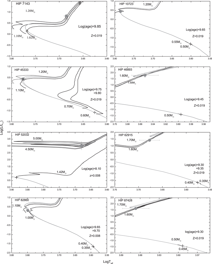
Figure 1. H–R diagrams of the eight systems. The black and gray lines represent the evolutionary tracks and the isochrone ages given by Girardi et al. (2000), respectively. The gray dots with error bars represent the positions of the primary with system luminosity. The cross and the plus symbols indicate the finally determined positions of primaries and secondaries, respectively. If the luminosity from the secondary can be ignored, the position of the primary is indicated only by the gray dots.
Download figure:
Standard image High-resolution imageThe orbital elements of the eight systems are given in Table 2 together with λ and ϖ. The semimajor axis of the secondary orbit relative to the primary can be expressed as

and the values are also given in Table 2. Additionally, the physical parameters of the components, including the masses (M1 and M2), the mass ratio q, the absolute visual magnitude of the system (MV), the luminosities (L1 and L2), the magnitude difference ( ) between the two components, the radii (R1 and R2), and the isochrone age, are listed in Table 3.
Table 2. The Fitting Results Including the Ratio (λ) of the Semimajor Axes Between the Photocentric and Primary Orbits, the Parallax (ϖ), and the Orbital Elements
| HIP | λ | ϖ | P | T | e | ω | K1 | i | Ω | a0 | a |
|---|---|---|---|---|---|---|---|---|---|---|---|
| Identifier | (mas) | (days) | (JD-2,450,000.0) | (deg) | (km s−1) | (deg) | (deg) | (mas) | (mas) | ||
| 7143 | 0.60 | 17.7 | 36.5191679 | 54094.8318 | 0.14286 | 203.34 | 35.861 | 65.0 | 47.05 | 1.6 | 3.40 |
| ± 0.5 | ± 0.00013 | ± 0.0075 | ± 0.00026 | ± 0.07 | ± 0.005 | ± 13.5 | ± 11.7 | ||||
| 10723 | 0.97 | 41.5 | 93.2874 | 54094.633 | 0.5217 | 103.87 | 19.655 | 105.1 | 281.0 | 6.0 | 19.5 |
| ± 0.4 | ± 0.0006 | ± 0.005 | ± 0.0002 | ± 0.03 | ± 0.005 | ± 3.5 | ± 3.1 | ||||
| 45333 | 0.94 | 50.2 | 16.23966 | 53400.083 | 0.10540 | 137.47 | 35.573 | 98.8 | 68.9 | 2.5 | 7.1 |
| ± 0.3 | ± 0.00001 | ± 0.001 | ± 0.00005 | ± 0.02 | ± 0.002 | ± 5.3 | ± 7.3 | 7.0 | |||
| 46893 | 1.00 | 8.2 | 822.5 | 53879.4 | 0.098 | 291.6 | 6.333 | 117.7 | 21.9 | 4.4 | 17.7 |
| ± 0.9 | ± 0.2 | ± 2.4 | ± 0.002 | ± 1.1 | ± 0.008 | ± 18.4 | ± 13.2 | ||||
| 52032 | 0.96 | 2.0 | 1500.10 | 54405.31 | 0.577 | 59.0 | 8.65 | 115.4 | 359.8 | 2.0 | 8.8 |
| ± 0.3 | ± 0.17 | ± 0.36 | ± 0.003 | ± 0.3 | ± 0.05 | ± 17.1 | ± 14.6 | ||||
| 62915 | 1.00 | 11.1 | 1010.5 | 53486.2 | 0.282 | 184.25 | 2.786 | 37.6 | 8.6 | 4.5 | 27.2 |
| ± 0.8 | ± 0.7 | ± 1.7 | ± 0.004 | ± 0.54 | ± 0.005 | ± 26.4 | ± 10.7 | ||||
| 82860 | 0.99 | 66.2 | 52.1089 | 53427.880 | 0.2221 | 338.46 | 17.465 | 90.5 | 23.5 | 5.3 | 20.0 |
| ± 0.2 | ± 0.0001 | ± 0.007 | ± 0.0002 | ± 0.05 | ± 0.004 | ± 2.2 | ± 2.0 | ||||
| 87428 | 1.00 | 9.6 | 467.52 | 54497.5 | 0.0042 | 251.5 | 4.013 | 144.9 | 171.4 | 2.9 | 14.6 |
| ± 0.5 | ± 0.07 | ± 19.5 | ± 0.0008 | ± 15.0 | ± 0.004 | ± 24.0 | ± 9.3 |
Note. The derived parameters (a0 and a) are also listed.
Download table as: ASCIITypeset image
Table 3.
The Obtained Physical Parameters of the Eight Binary Systems Including the Component Masses (M1 and M2), the Mass Ratio q, the Absolute Visual Magnitudes MV of the System, the Component Luminosities (L1 and L2), the Magnitude Difference  the Component Radii (R1 and R2), and the Isochrone Ages
| HIP | M1 | M2 | q | MV | L1 | L2 |

|
R1 | R2 | log(age yr−1) |
|---|---|---|---|---|---|---|---|---|---|---|
| Identifier |

|

|

|

|

|

|
||||
| 7143 | 1.14 | 1.02 | 0.89 | 3.02 | 5.40 | 1.41 | 1.46 | 3.3 | 1.2 | 9.86 |
| 10723 | 1.20 | 0.53 | 0.45 | 3.69 | 2.76 | 0.04 | 4.60 | 1.5 | 0.4 | 9.65 |
| 45333 | 1.12 | 0.61 | 0.55 | 3.68 | 2.71 | 0.09 | 3.70 | 1.5 | 0.6 | 9.78 |
| 46893 | 1.51 | 0.50 | 0.33 | 0.82 | 63.57 | 0.04 | 8.00 | 13.2 | 0.4 | 9.45 |
| 52032 | 4.94 | 1.42 | 0.29 | −2.07 | 1296.36 | 5.89 | 5.86 | 53.7 | 1.4 | 8.10 |
| 62915 | 1.62 | 0.39 | 0.24 | 1.67 | 26.66 | 0.02 | 7.81 | 7.6 | 0.3 | 9.33 |
| 82860 | 1.04 | 0.37 | 0.35 | 3.98 | 2.02 | 0.02 | 5.01 | 1.2 | 0.3 | 9.67 |
| 87428 | 1.66 | 0.41 | 0.25 | 1.20 | 42.50 | 0.03 | 7.88 | 10.1 | 0.4 | 9.29 |
Download table as: ASCIITypeset image
3.2. HIP 7143 and HIP 45333
Among the eight systems, we find that only HIP 7143 and 45333 have relatively small component magnitude differences. Specifically, this suggests that only the secondaries of the two systems can be resolved by the present-day observational techniques. Actually, the two systems have been recently resolved using the spectroscopic observations and transformed into SB2s (Halbwachs et al. 2011, 2012, 2014; Fekel et al. 2015).
For HIP 7143, the estimated mass ratio is 0.88, which is slightly larger than the value 0.7624 derived from the RVD of both the primary and secondary (Halbwachs et al. 2014). From Figure 1, we see that the primary has evolved away from the main sequence and is now a giant star, while the secondary is still on the main sequence. As a result, the primary is much brighter than one would expect from the mass–luminosity relation for main sequence stars. This is probably the reason why there are only six radial velocity measurements for the secondary. In order to get a high-quality spectroscopic orbit of the secondary, further observations with the latest techniques are needed.
From Figure 1, we find that both component stars of HIP 45333 are on the main sequence. This system was regarded as an SB1 before 2015. With a large number of new spectroscopic observations for both the primary and the secondary, a spectroscopic orbit more accurate than the previous one (Katoh et al. 2013) was determined by Fekel et al. (2015). Also, fixing the spectroscopic orbital elements, Fekel et al. (2015) derived the astrometric orbit by fitting the HIAD. The physical properties based on these orbital solutions are in accordance with ours. Further improvement to the astrometric orbit will rely on the interferometric data or the Gaia astrometric data.
Besides the revised HIAD and RVD mentioned above, the double-lined spectroscopic data are added to determine the orbital solutions of HIP 7143 and HIP 45333 on the basis of the iterative method developed in this work. Then Equation (4) can be rewritten as

where  and
 indicate the RVD and the corresponding error of the secondary, respectively. The integer N3 is the number of the RVD of the secondary. The derived orbital solutions and the dynamical masses of the component stars are listed in Table 4. We find that the dynamical masses of the component stars are in accordance with the values relying on the evolutionary model and those given by Fekel et al. (2015) for HIP 45333.
Table 4. The Orbital Elements of HIP 7143 and HIP 45333 With Double-lined Spectroscopic Data Added
| Elements | HIP 7143 | HIP 45333 |
|---|---|---|
| λ | 0.63 | 0.93 |
| ϖ | 17.7 ± 0.5 | 50.2 ± 0.3 |
| P(days) | 36.5192 ± 0.0001 | 16.239659 ± 0.000004 |
| T(JD-2,450,000.0) | 54094.832 ± 0.008 | 53400.084 ± 0.001 |
| e | 0.1429 ± 0.0003 | 0.10566 ± 0.00005 |
| ω(deg) | 203.34 ± 0.07 | 137.45 ± 0.02 |
| K1 (km s−1) | 35.581 ± 0.005 | 35.895 ± 0.002 |
| K2 (km s−1) | 46.079 ± 0.994 | 65.89 ± 0.22 |
| i (deg) | 65.4 ± 13.3 | 99.0 ± 5.3 |
| Ω(deg) | 47.5 ± 11.4 | 69.9 ± 7.4 |
| a0(mas) | 1.4 | 2.5 |
| a(mas) | 3.0 | 5.2 |
M1( ) |
1.49 ± 0.48 | 1.17 ± 0.05 |
M2( ) |
1.16 ± 0.37 | 0.64 ± 0.03 |
Download table as: ASCIITypeset image
4. CONCLUSIONS
An iterative method is developed to determine the self-consistent orbital solutions of SB1s along with compatible physical properties of component stars via a simultaneous fit including both the revised HIAD and RVD. Applying this method, we obtain reliable orbital solutions of eight systems. It is valuable to apply the method to all the SB1s in the 9th Catalog of Orbits of Spectroscopic Binaries (Pourbaix et al. 2004) and pick out the ones with a small component magnitude difference as the preferred sample for further observations.
As is known to all, the Gaia mission is running now and its astrometric data with precision much higher than Hipparcos will soon be available. By fitting these data, orbits can be obtained for nearly all the existing SB1s. For those SB1s with high signal-to-noise ratio, one can directly fit the Gaia astrometric data to give the astrometric orbits and λ, and then give the physical properties of the components. But for those SB1s with low signal-to-noise ratios, similar to the situation in this work, the method developed here is more suitable.
This research has made use of the SIMBAD astronomical literature database, operated at CDS, Strasbourg, France. We would like to thank an anonymous referee for instructive remarks, particularly those on the simultaneous fit including both the revised HIAD and the radial velocity data. This research is supported by the National Natural Science Foundation of China under grant Nos. 11073059, 10833001, 11178006, 11273066, and 11203086.


