Simulation of Comet-Solar Wind Interaction in the AMROC Framework with the IGLM-MHD Scheme

Abstract

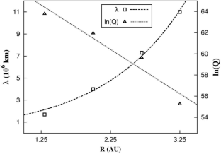
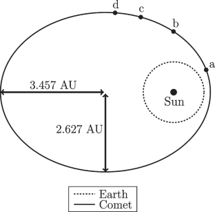
In this work we present 2-dimensional, 1-fluid magnetohydrodynamic (MHD) simulations of the interaction of a comet with the solar wind. Even though our model can in principle run simulations with time-dependent physical parameters representing the comet travelling along its elliptic orbit, here we focus on “snapshots” at four heliocentric distances, namely: 1.3, 2.0, 2.7 and 3.25 AU. This strategy allows us to analyse some key features of the comet at relatively low computational cost. Our aim here is to present our implementation of such a scenario with the AMROC computational code and study the main features of the comet, which has the physical characteristics of 67P/Churyumov-Gerasimenko (67P/CG). The dependence of the physical parameters on the heliocentric distance is given by means of Parker’s model and of functions obtained from curve fitting of data collected in the literature. In addition, we model comets with three forms: circular, elliptic and bilobed (or “peanut-shaped”.) AMROC is in development and the model shown here is an valuable contribution to these efforts, as it represents a new kind of problem implemented in this code. Furthermore, our model provides the possibility of creation of new and interesting scenarios with regard to comets and other sources of plasma.

Appendices

Appendix A: On the normalized units used in this paper

We use a normalization scheme such that the original CGS values of mass m, time t and length l are converted into new dimensionless ones ($m_{\text {\tiny {N}}}$, $t_{\text {\tiny {N}}}$ and $l_{\text {\tiny {N}}}$) by

$$\begin{aligned} \begin{aligned} m_{\text {\tiny {N}}}&=\frac{m}{10^{-23+3\delta }{g}},\\ t_{\text {\tiny {N}}}&=\frac{t}{10^{(-13+2\delta )/2}{s}},\\ l_{\text {\tiny {N}}}&=\frac{l}{10^{\delta }~\text {cm}}, \end{aligned} \end{aligned}$$

(A1)

where the appropriate value of $\delta$ is defined for each case, bearing in mind the size of the domain.

With the units given by (A1), the density $\rho$, pressure p and the components $B_{j}$ of the magnetic field are normalized in the following way:

$$\begin{aligned} \begin{aligned} \rho _{\text {\tiny {N}}}&=\frac{\rho }{10^{-23}{g\, \text {cm}^{-3}}}, \\ p_{\text {\tiny {N}}}&=\frac{p}{10^{-10}{g\,\text {cm}^{-1}\,s^{-2}}}, \\ B_{j}^{\text {\tiny {N}}}&=\frac{B_{j}}{10^{-5}{G}}. \end{aligned} \end{aligned}$$

(A2)

In addition, the magnetic permeability assumes the value $\mu ^{\text {\tiny {N}}}_{0}=4\pi$.

Appendix B: Accuracy Verification of the SAMR Implementation

Deiterding [21] presents a two-dimensional test created to verify the accuracy and the order of convergence of the SAMR scheme and compare them with the ones for uniform grid simulations. This test consists in a simulation in a computational domain $\Omega =[-1,1]^2$ with periodic boundary conditions at all borders. Regarding the physical conditions, the density $\rho$ has the initial profile given by the Gaussian function

$$\begin{aligned} \rho _{0}(x,y)=1+\textrm{e}^{-(x^2+y^2)/\sigma ^2} , \end{aligned}$$

(B3)

with $\sigma =0.25$. On the other hand, the initial values of velocity and pressure are given respectively by $\textbf{v}=(1,1)$ and $p_0=1$. The simulation runs until the maximum time of $t_\textrm{max}=2$, when the initial conditions are replicated, and this provides a straightforward way to calculate the error norms on uniform grids.

Here, Deiterding uses the $L_1$-error, evaluated for $\rho$ by means of the expression

$$\begin{aligned} L_1(\rho )=L_1(\Delta x_{\,l_\textrm{max}},\Delta y_{\, l_\textrm{max}},G_{l_\textrm{max}})+\sum ^{l_\textrm{max}-1}_{l=0}L_1(\Delta x_{\,l},\Delta y_{\,l},G_{l}\setminus G_{l+1}), \end{aligned}$$

(B4)

where $l_\textrm{max}$ labels the highest level of refinement and $G_{l}$ is the domain of level l (Section 4.) In addition, in Eq. (B4)

$$\begin{aligned} L_{1}(\Delta x, \Delta y, \cdot )=\sum ^{l}_{i,j}|\rho _{ij}-\rho _{0}(x^{i}_{l},y^{j}_{l})|\Delta x_{\,l}\Delta y_{\,l}. \end{aligned}$$

(B5)

That is, $L_1(\Delta x, \Delta y, \cdot )$ is the error norm on a sub-domain of level l. Note that, in the SAMR case, (B4) is calculated on each $G_{l}$ without considering higher levels of refinement. More details can be found in [21].

Figure 13 shows the $L_1$-errors and the respective orders of convergence for the aforementioned simulation for two cases: with uniform grid and with the SAMR implementation. The last runs with two levels of refinement and $r=2$ (see Section 4). Each entry in the x-axis refers to a domain with $N^2$ cells for the uniform grid. In the SAMR case, even if the simulation starts with $N=20$, we have at most $N=80$ after two levels of refinement. Therefore, for the SAMR cases, there is no data for $N=20$ and 40. The order of convergence is defined by $\log _2(L^k_1/L^{k+1}_1)$, where the integer $k\geqslant 1$ denotes the position in the x-axis, with $k=1$ corresponding to $N=20$. In addition, it is analysed the role of the conservative flux correction (“fixup”, see details in Section 2.1.6 of [21]) in the SAMR simulations.

Fig. 13

Upper diagram: $L_{1}$-Error norm for uniform grid, SAMR with fixup and SAMR without fixup; lower panel: Order of convergence for the same three cases

As observed by Deiterding, the absolute errors for the SAMR case are slightly higher than in the uniform grid. However, in all cases the errors decrease as N increases, which indicates convergence. Without fixup, the errors (order) become slightly higher (lower) than in the situation with fixup.

Still according to Deiterding, a second-order accurate method can be inferred from the values of the order of convergence, even in the SAMR cases. Furthermore, note that the uniform grid simulation has the higher order of convergence for the highest resolution.

Appendix C: Elliptic and Bilobed Comets

1.1 C.1 Elliptic Comet

We start with the elliptic coordinates given by

$$\begin{aligned} \begin{aligned} x&= \xi \cosh \mu \cos \nu \;, \\ y&= \xi \sinh \mu \sin \nu \;, \end{aligned} \end{aligned}$$

(C6)

and their inverse

$$\begin{aligned} \begin{aligned} \mu&= {{\,\textrm{arccosh}\,}}\left[ \frac{\sqrt{(x+\xi )^2+y^2}+\sqrt{(x-\xi )^2+y^2}}{2\xi }\right] \; , \\ \nu&= \arccos \left[ \frac{\sqrt{(x+\xi )^2+y^2}-\sqrt{(x-\xi )^2+y^2}}{2\xi }\right] . \end{aligned} \end{aligned}$$

(C7)

The above equations represent a family of confocal ellipses where the foci are at $-\xi$ and $\xi$ on the x-axis. In (C6) and (C7), $\nu \in [0,2\pi )$ and each value of $\mu \geqslant 0$ corresponds to an ellipse with eccentricity $e=1/\cosh \upmu$ ($\upmu =0$ is the degenerate case). Therefore, each point (x, y) of the domain belongs to one and only one ellipse, whose properties are worked out as follows: a point (x, y) is given; $\upmu$ (and therefore e) is calculated with the first of (C7); the semi-major and semi-minor axes are then given by $a=\xi /e$ and $b=\xi \sqrt{1-e^2}/e$, respectively. Note that $\alpha$ is constant and is defined for each object being simulated.

Now, for each point (x, y) we can calculate the velocity field $\mathbf {u_n}(x,y)$ around the comet, in the form

$$\begin{aligned} \mathbf {u_n}(x,y)=|\mathbf {u_{n}}|~\frac{\nabla f(x,y)}{|\nabla f(x,y)|}, \end{aligned}$$

(C8)

where $f(x,y)=e^2x^2/\xi ^2+e^2y^2/[\xi ^2(1-e^2)]-1$. The velocity $\textbf{v}$ in (4) and (6) is treated similarly.

On the other hand, we must adapt (5) to elliptic comets, once it was originally intended for spherical sources. Here we propose a simple approach: we interpret r as the average value of the radial coordinate of the ellipse with center at the origin, that is,

$$\begin{aligned} r~:= \overline{r}(e)=\frac{a}{2\pi }\int ^{2\pi }_{0}\sqrt{\frac{(1-e^2)}{1-e^2\cos ^2(\theta )}}\ d\theta = \frac{a}{2\pi }I(e). \end{aligned}$$

(C9)

With this, for each point (x, y) we have an defined value of  $\overline{r}(e)$. Unfortunately, (C9) does not have a solution in terms of elementary functions for $e \ne 0$. However, by numerical integration, we can calculate I(e) for prescribed values of e and perform a curve fitting of the data to obtain an expression for $\overline{r}(e)$. Table 3 shows the selected values of e and their corresponding I(e).

Table 3 The integral I(e) of (C9) calculated for some values of e

The 4th degree polynomial

$$\begin{aligned} I(e)=-30.789 e^4+51.206 e^3-30.283 e^2+5.810 e+5.974 \end{aligned}$$

(C10)

is a good fit for the data of Table 3 in the interval $e \in [0,1)$, giving 0.22561 and 0.0150407 for the final sum of the squares of residuals and the reduced chi-squares, respectively¹.

Finally, we must bear in mind that, in our model, Eq. (C8) is not calculated inside the object, that is, it is only valid if the following condition is satisfied:

$$\begin{aligned} \sqrt{x^2+\frac{y^2}{1-e_\textrm{com}^2}}\;\geqslant \;a_\textrm{com}, \end{aligned}$$

(C11)

where $e_\textrm{com}$ and $a_\textrm{com}$ are, respectively, the eccentricity and the semi-major axis of the comet.

1.2 C.2 Bilobed Comet

We employ the polar equation $r(\theta )=p\rho +q\cos (2\theta )$, where the radial coordinate $r(\theta )$ is measured from the origin, p and q are constants and $\rho \in [1,\infty )$. This equation describes a family of concentric curves (one for each value of $\rho$) that intersect the x-axis and the y-axis at $(\pm \alpha ,0)$ and $(0,\pm \beta )$, where $\alpha =p\rho +q$ and $\beta =p\rho -q$. Note that the bilobed curves become more circular, that is, $\alpha \approx \beta \approx p\rho$ for $\rho \gg 1$. On the other hand, in our model the surface of the comet corresponds to $\rho =1$ by definition, such that the parameters a and b (which define the dimensions of the object) are $\alpha _\textrm{com}=p+q$ and $\beta _\textrm{com}=p-q$.

From the aforementioned polar equation, we can deduce the parametric equations

$$\begin{aligned} \begin{aligned} x&= [p\rho +q\cos (2\theta )]\cos \theta , \\ y&= [p\rho +q\cos (2\theta )]\sin \theta , \end{aligned} \end{aligned}$$

(C12)

and their inverses, in the form

$$\begin{aligned} \begin{aligned} \rho&= \frac{1}{p}\sqrt{x^2+y^2}-\frac{q}{p}\left( \frac{x^2-y^2}{x^2+y^2}\right) , \\ \theta&= \arctan \left( \frac{y}{x}\right) . \end{aligned} \end{aligned}$$

(C13)

The initial velocity field of the ejected plasma is calculated with (C8) and $f(r,\theta )=r-p\rho -q\cos (2\theta )$. With this and (C13), we obtain

$$\begin{aligned} \textbf{u}(x,y)=\frac{u_0}{|\nabla f(x,y)|}\left\{ \left[ \frac{x}{r}-\frac{2(\alpha -\beta )xy^2}{r^4}\right] \hat{\textbf{x}}+\left[ \frac{y}{r}+\frac{2(\alpha -\beta )x^2y}{r^4}\right] \hat{\textbf{y}}\right\} , \end{aligned}$$

(C14)

where

$$\begin{aligned} |\nabla f(x,y)|=\left\{ 1+\left[ \frac{2(\alpha -\beta )xy}{r^3}\right] ^2\right\} ^{1/2}, \end{aligned}$$

(C15)

and $r=(x^2+y^2)^{1/2}$. Note that Eqs. (C14) and (C15) are written in the more convenient parameters $\alpha$ and $\beta$.

As in the previous case, $\mathbf {u_n}(x,y)$ is not calculated inside the body. With this and bearing in mind that $\alpha _\textrm{com}$ and $\beta _\textrm{com}$ can be related by $\alpha _\textrm{com}=c\beta _\textrm{com}$ where c is a constant, the condition of validity of Eq. (C14) is

$$\begin{aligned} \frac{c(x^2+y^2)^{3/2}}{cx^2+y^2}\;\geqslant \;\alpha _\textrm{com}. \end{aligned}$$

(C16)

Regarding the calculation of (5), we again consider r as the average value of $r(\theta )$ over $[0,2\pi )$, that is,

$$\begin{aligned} r :=\overline{r}=\frac{1}{2\pi }\int ^{2\pi }_{0}[p\rho +q\cos (2\theta )]d\theta =\rho \frac{\alpha +\beta }{2}. \end{aligned}$$

(C17)

As an example, the left panel of Fig. 14 shows the vector field of $\mathbf {u_n}(x,y)$ for an ellipse with $e_\textrm{com}=0.9$ and $a_\textrm{com}=0.25$, in normalized units. In the right panel we have the bilobed form, with $\alpha _\textrm{com}=0.25$ and $\beta _\textrm{com}=\alpha _\textrm{com}/3$.

Fig. 14

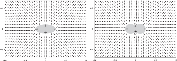
Left: vector field of $\mathbf {u_n}(x,y)$ for the elliptic case, with $\mathbf {u_n}(x,y)$ for $e_\textrm{com}=0.9$. Right: the same for the bilobular case with $\alpha _\textrm{com}=0.25$ and $\beta _\textrm{com}=\alpha _\textrm{com}/3$

References

J.M. Greenberg, Making a comet nucleus. Astron. Astrophys. 330(1), 375–380 (1998)
H. Gunnel, I. Mann, C.S. Wedlund, E. Kallio, M. Alho, H. Nilsson, J. De Keyser, F. Dhooghe, R. Maggiolo, Acceleration of ions and nano dust at a comet in the solar wind. Planet. Space Sci. 119, 13–23 (2015). https://doi.org/10.1016/j.pss.2015.08.019
D.A. Ostlie, B.W. Carroll, An Introduction to Modern Astrophysics, 2nd edn. (Addison-Wesley Publishing Company Inc, Boston, USA, 1996)
M. Harwit, Astrophysical Concepts, 3rd edn. (Springer-Verlag, New York, USA, 1998)
L. Biermann, B. Brosowski, H.U. Schmidt, The interaction of the solar wind with a comet. Sol. Phys. 1(2), 254–284 (1967). https://doi.org/10.1007/BF00150860
D.T. Young, F.J. Crary, J.E. Nordholt, F. Bagenal, D. Boice, J.L. Burch, A. Eviatar, R. Goldstein, J.J. Hanley, D.J. Lawrence, D.J. McComas, R. Meier, D. Reisenfeld, K. Sauer, R.C. Wiens, Solar wind interactions with Comet 19P/Borrelly. Icarus 167(1), 80–88 (2004). https://doi.org/10.1016/j.icarus.2003.09.011
L. Matteini, S.J. Schwartz, P. Hellinger, Cometary ion instabilities in the solar wind. Planet. Space Sci. 119, 3–12 (2015). https://doi.org/10.1016/j.pss.2015.08.016
V.B. Baranov, M.G. Lebedev, The interaction between the solar wind and the comet P/Halley atmosphere: observations versus theoretical predictions. Astron. Astrophys. 273, 695–706 (1993)
K. Murawski, D.C. Boice, W.F. Huebner, C.R. DeVore, Two-dimensional MHD simulations of the solar wind interaction with Comet Halley. Acta Astronom. 48(4), 803–817 (1998)
R. Wegmann, The effect of some solar wind disturbances on the plasma tail of a comet: models and observations. Astron. Astrophys. 358(2), 759–775 (2000)
A.P. Rasca, R. Oran, M. Horányi, Mass loading of the solar wind by a sungrazing comet. Geophys. Res. Lett. 41(15), 5376–5381 (2015). https://doi.org/10.1002/2014GL060990
J. Deca, A. Divin, P. Henri, A. Eriksson, S. Markidis, V. Olshevsky, M. Horányi, Electron and ion dynamics of the solar wind interaction with a weakly outgassing comet. Phys. Rev. Lett. 118(20), 205,101 (2017). https://doi.org/10.1103/PhysRevLett.118.205101
M. Stefano, G. Lapenta, Rizwan-uddin, Multi-scale simulations of plasma with iPIC3D. Math. Comput. Simul. 80(7), 1509–1519 (2010). https://doi.org/10.1016/j.matcom.2009.08.038
C. Koenders, C. Perschke, C. Goetz, I. Richter, U. Motschmann, K.-H. Glassmeier, Low-frequency waves at comet 67P/Churyumov-Gerasimenko. Observations compared to numerical simulations. Astron. Astrophys. 594(A66), 1–16 (2016). https://doi.org/10.1051/0004-6361/201628803
J. Müller, S. Simon, U. Motschmann, J. Schüle, K.-H. Glassmeier, G.J. Pringle, A.I.K.E.F., Adaptive hybrid model for space plasma simulations. Comput. Phys. Commun. 182(4), 946–966 (2011). https://doi.org/10.1016/j.cpc.2010.12.033
K.-H. Glassmeier, H. Boehnhardt, D. Koschny, E. Kührt, I. Richter, The Rosetta Mission: Flying towards the origin of the Solar System. Space Sci. Rev. 128, 1–21 (2007). https://doi.org/10.1007/s11214-006-9140-8
M. Rubin, C. Koenders, K. Altwegg, M.R. Combi, K.-H. Glassmeier, T.I. Gombosi, K.C. Hansen, U. Motschmann, I. Richter, V.M. Tenishev, G. Tóth, Plasma environment of a weak comet – Predictions for Comet 67P/Churyumov–Gerasimenko from multifluid-MHD and Hybrid models. Icarus 242(A66), 38–49 (2014). https://doi.org/10.1016/j.icarus.2014.07.021
K.G. Powell, P.L. Roe, T.J. Linde, T.I. Gombosi, D.L. DeZeeuw, A solution-adaptive upwind scheme for ideal magnetohydrodynamics. J. Comp. Phys. 154(2), 284–309 (1999). https://doi.org/10.1006/jcph.1999.6299
Z. Huang, G. Tóth, T.I. Gombosi, X. Jia, M. Rubin, N. Fougere, V. Tenishev, M.R. Combi, A. Bieler, K.C. Hansen, Y. Shou, K. Altwegg, Four-fluid MHD simulations of the plasma and neutral gas envinment of comet 67P/Churyumov-Gerasimenko near perihelion. J. Geophys. Res. Space Physics 121, 4247–4268 (2016). https://doi.org/10.1002/2015JA022333
E.F.D. Evangelista, M.O. Domingues, O. Mendes, O.D. Miranda, A brief study of instabilities in the context of space magnetohydrodynamic simulations. Rev. Bras. Ensino Fis. 38(1), 130,91-130,913 (2016). https://doi.org/10.1590/S1806-11173812098
R. Deiterding, Block-structured adaptive mesh refinement - theory, implementation and application. ESAIM Proc. 34(1), 97–150 (2011). https://doi.org/10.1051/proc/201134002
V.B. Baranov, D.B. Alexashov, M.G. Lebedev, MHD simulation of the solar wind flow around the coma of comet Churyumov-Gerasimenko during Rosetta’s flyby. Mon. Not. R. Astron. Soc. 482(4), 5642–5650 (2019). https://doi.org/10.1093/mnras/sty3080
T. Yokoyama, K. Shibata, Magnetohydrodynamic simulation of a solar flare with chromospheric evaporation effect based on the magnetic reconnection model. Atrophys. J. 549, 1160–1174 (2001). https://doi.org/10.1086/319440
M. González-Servín, J.J. González-Avilés, Numerical mhd simulations of solar flares and their associated small-scale structures. Mon. Not. R. Astron. Soc. 528, 5098–5113 (2024). https://doi.org/10.1093/mnras/stae375
T.I. Gombosi, D.L. DeZeeuw, R.M. Häberli, K.G. Powell, Three-dimensional multiscale MHD model of cometary plasma environments. J. Geophys. Res. 101(A7), 15233–15253 (1996). https://doi.org/10.1029/96JA01075
T.I. Gombosi, K.C. Hansen, D.L. DeZeeuw, M.R. Combi, K.G. Powell, MHD simulation of comets: The plasma environment of comet Hale-Bopp. Earth Moon Planets 79, 179–207 (1997). https://doi.org/10.1023/A:1006289418660
L. Haser, Distribution d’intensité dans la tête d’une comète. Bull. Soc. Roy. Sci. Liège 43, 740–750 (1957)
C. Koenders, K.-H. Glassmeier, I. Richter, H. Ranocha, U. Motschmann, Dynamical features and spatial structures of the plasma interaction region of 67P/Churyumov-Gerasimenko and the solar wind. Planet. Space Sci. 105(Suppl. C), 101–116 (2015). https://doi.org/10.1016/j.pss.2014.11.014
K.C. Hansen, T. Bagdonat, U. Motschmann, C. Alexander, M.R. Combi, T.E. Cravens, T.I. Gombosi, Y.-D. Jia, I.P. Robertson, The plasma environment of comet 67P/Churyumov-Gerasimenko throughout the Rosetta main mission. Space Sci. Rev. 128(1–4), 133–166 (2007). https://doi.org/10.1007/s11214-006-9142-6
E.N. Parker, Dynamics of the interplanetary gas and magnetic fields. Astrophys. J. 128, 664–676 (1958). https://doi.org/10.1086/146579
R.C. Tautz, A. Shalchi, A. Dosch, Simulating heliospheric and solar particle diffusion using the Parker spiral geometry. J. Geophys. Res. Space Physics 116(A2), A02,102 (2011). https://doi.org/10.1029/2010JA015936
H.-Q. He, New insight into the formation mechanism of the energetic particle reservoirs in the heliosphere. MNRAS 508(1), L1–L5 (2021). https://doi.org/10.1093/mnrasl/slab094
A. Ekenbäck, M. Holmström, S. Barabash, H. Gunell, Energetic neutral atom imaging of comets. Geophys. Res. Lett. 35(5), L05,103 (2008). https://doi.org/10.1029/2007GL032955
M. Maksimovic, S.D. Bale, L. Berčič, J.W. Bonnell, A.W. Case, T.D. de Wit, K. Goetz, J.S. Halekas, P.R. Harvey, K. Issautier, 18 more authors, Anticorrelation between the bulk speed and the electron temperature in the pristine solar wind: First results from the Parker Solar Probe and comparison with Helios. Astrophys. J. Suppl. S. 246, 62 (2020). https://doi.org/10.3847/1538-4365/ab61fc
H. Goldstein, C. Poole, J. Safko, Classical Mechanics, 3rd edn. (Addison-Wesley Publishing Company Inc, Boston, USA, 2001)
The International Astronomical Union. Minor Planet Center (2023). http://www.minorplanetcenter.net/db_search/show_object?object_id=67P
E.F. Toro, Riemann solvers and numerical methods for fluid dynamic - A practical introduction, 3rd edn. (Springer-Verlag, Berlin, Heidelberg, 2009)
T. Miyoshi, K. Kusano, A multi-state HLL approximate Riemann solver for ideal magnetohydrodynamics. J. Comp. Phys. 208(1), 315–344 (2005). https://doi.org/10.1016/j.jcp.2005.02.017
A. Harten, P.D. Lax, B. van Leer, On upstream differencing and Godunov-type schemes for hyperbolic conservation laws. SIAM Rev. 25(1), 35–61 (1983). https://doi.org/10.1137/1025002
D. Derigs, A.R. Winters, G.J. Gassner, S. Walch, M. Bohm, Ideal GLM-MHD: about the entropy consistent nine-wave magnetic field divergence diminishing ideal magnetohydrodynamics equations. J. Comp. Phys. 364, 420–467 (2018). https://doi.org/10.1016/j.jcp.2018.03.002
A. Mignone, P. Tzeferacos, A second-order unsplit Godunov scheme for cell-centered MHD: the CTU-GLM scheme. J. Comp. Phys. 229, 2117–2138 (2010). https://doi.org/10.1016/j.jcp.2009.11.026
A. Dedner, F. Kemm, D. Kröner, C.-D. Munz, T. Schnitzer, M. Wesenberg, Hyperbolic divergence cleaning for the MHD equations. J. Comp. Phys. 175, 645–673 (2002). https://doi.org/10.1006/jcph.2001.6961
L.S. Cassara, M.M. Lopes, M.O. Domingues, O. Mendes, R. Deiterding, On thermodynamic consistency of generalised Lagrange multiplier magnetohydrodynamic solvers. Comp. Appl. Math. 42, 223 (2023). https://doi.org/10.1007/s40314-023-02338-2
M.M. Lopes, R. Deiterding, A.K.F. Gomes, O. Mendes, M.O. Domingues, An ideal compressible magnetohydrodynamic solver with parallel block-structured adaptive mesh refinement. Comp. Fluids 173, 293–298 (2018). https://doi.org/10.1016/j.compfluid.2018.01.032
K.-H. Glassmeier, Interaction of the solar wind with comets: a Rosetta perspective. Phil. Trans. R. Soc. A 375(2097), 20160256 (2017). https://doi.org/10.1098/rsta.2016.0256
M.M. Lopes, R. Deiterding, M.O. Domingues, O. Mendes, in Civil-Comp Conferences, Proceedings of the Eleventh International Conference on Engineering Computational Technology, vol. 2, ed. by B.H.V. Topping, P. Iványi (Civil-Comp Press, Edinburgh, UK, 2022), p. 2.8
M.M. Lopes, Numerical methods applied to space magnetohydrodynamics for high performance computing. Doctorate thesis, National Institute for Space Research. (São José dos campos, Brazil, 2019). http://mtc-m21c.sid.inpe.br/col/sid.inpe.br/mtc-m21c/2019/04.02.23.51/doc/publicacao.pdf
Acknowledgements
The authors acknowledge INPE for providing the necessary computer resources and AEB for scientific support.
Funding
EFDE acknowledges Conselho Nacional de Desenvolvimento Científico e Tecnológico (CNPq, PCI/INPE Program, grants 301229/2023-6 and 301351/2024-4). LC acknowledges CNPq, grant 140563/2020-2. VEM acknowledges CNPq (PCI/INPE Program, grants 400077/2022-1, Proc. 316374/2025-3). The authors also acknowledge financial support from FAPESP Project 2020/13015-0.
Author information
Authors and Affiliations
Contributions
E.F.D.E. wrote the manuscript, prepared the model to be simulated and generated the results, under supervision of O.M., M.O.D. and O.D.M.; L.C. revised the text and improved the discussion on the IGLM scheme, besides giving pertinent suggestions in other sections of the paper. V.E.M. greatly contributed to the computational work, helping E.F.D.E. to handle tricky implementation and runtime problems. R.D. is the creator of AMROC, which is the computational code used in the simulations presented in this manuscript. Furthermore, R.D. carefully revised the text, made adjustments to it and gave important insights.
Corresponding author
Ethics declarations
Competing interests
The authors declare no competing interests.
Additional information
Publisher's Note
Springer Nature remains neutral with regard to jurisdictional claims in published maps and institutional affiliations.