<?xml version="1.0" encoding="utf-8"?>
<feed xmlns="http://www.w3.org/2005/Atom">

    <title>
        Chris Stucchio
    </title>

    <link href="http://www.chrisstucchio.com/blog/atom.xml" rel="self" />
    <link href="https://www.chrisstucchio.com"/>

    <updated>2023-04-02T05:57:55.076445Z</updated>

    <id>https://www.chrisstucchio.com/</id>

        <entry>
            <title type="html">Boosting as a scheme for transfer learning</title>
            <author><name>Chris Stucchio</name></author>
            <link href="https://www.chrisstucchio.com/blog/2022/boosting_for_knowledge_transfer.html?utm_medium=rss&amp;utm_source=rss&amp;utm_campaign=rss"/>
            <updated>2022-12-29T08:30:00+01:00Z</updated>
            <published>2022-12-29T08:30:00+01:00Z</published>
            <id>https://www.chrisstucchio.com/blog/2022/boosting_for_knowledge_transfer.html</id>

            <content type="html">
              <![CDATA[
                (If mathematical formulas are not showing up here, <a href="https://www.chrisstucchio.com/blog/2022/boosting_for_knowledge_transfer.html?utm_medium=rss&amp;utm_source=rss&amp;utm_campaign=rss">please read this on the web.</a>.)
                <p>Here's a scenario that I believe to be common. I've got a dataset I've been collecting over time, with features <span class="math">\(x_1, \ldots, x_m\)</span> This dataset
will generally represent decisions I want to make at a certain time. This data is not a timeseries, it's just data I happen to have collected over time. I will call this the <em>old data</em> and <em>old features</em>.</p>
<p>The problem I'm interested in right now is the situation where some of the data was not collected since the beginning of time. I will assume that on a much smaller dataset - e.g. the most recent 10-20% of the data - I have collected additional features <span class="math">\(x_{m+1} \ldots x_m\)</span> which I have reason to believe are useful for predictions.
I will call this the <em>new data</em> and <em>new features</em>.</p>
<p>The challenge here is that if we combine the training data into a single table, it looks something like this:</p>
<table>
<thead>
<tr>
<th>x1</th>
<th>x2</th>
<th>Xn+1</th>
<th>Xn+2</th>
<th>y</th>
</tr>
</thead>
<tbody>
<tr>
<td>5</td>
<td>-3</td>
<td>null</td>
<td>null</td>
<td>False</td>
</tr>
<tr>
<td>7</td>
<td>2</td>
<td>null</td>
<td>null</td>
<td>True</td>
</tr>
<tr>
<td>.</td>
<td>0</td>
<td>.</td>
<td>.</td>
<td>.</td>
</tr>
<tr>
<td>3</td>
<td>5</td>
<td>0.2</td>
<td>-0.5</td>
<td>False</td>
</tr>
<tr>
<td>4</td>
<td>-6</td>
<td>0.9</td>
<td>1.2</td>
<td>True</td>
</tr>
</tbody>
</table>
<p>This dataset is not representative of future data; future data will not have nulls in the columns representing the new features.</p>
<p>It is my desire to build a scheme for transfer learning using non-neural network methods such as <a href="https://xgboost.readthedocs.io/en/stable/">XGB</a>. Specifically,
I want to train a model on the large dataset using only the old features, then transfer knowledge gained in this way to a model trained on the small dataset and
including the new features. In this blog post I provide a proof of concept on that <a href="https://en.wikipedia.org/wiki/AdaBoost">classical boosting</a> provides
a mechanism for accomplishing this knowledge transfer.</p>
<p><strong>Concrete example:</strong> standard stock market data, e.g. end of day prices, along with data pulled out of assorted EDGAR documents. This data is generally available
as far back as I'd like, provided I'm willing to parse old SEC files or pay a data provider for it. I also have some alternative data which only goes back a
couple of years. I believe it is customary to pretend this is satellite photos of cars in walmart parking lots rather than badly anonymized data about consumers
purchased from VISA or T-Mobile which consumers would generally expect to be kept confidential.</p>
<p>Standard options include:</p>
<ol>
<li>Training a model on all rows, including rows for which the new data is null.</li>
<li>Training a model only on the new data.</li>
</ol>
<p>
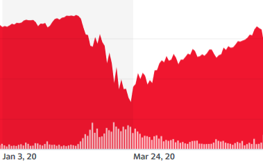
A significant problem with (1) is that the model can learn spurious correlations between missingness and outcomes - e.g. if one starts collecting new data
during a bear market, the model may learn "data present = stonks go down". The key problem with (2) is that the size of the new dataset might just be too
small.</p>
<h2>Alternate setup: Trunk and Branch Models</h2>
<p>Another way to think about this setup for the dataset is via the concept of "trunk and branch" models. One has a large dataset - in the neural
network context this is typically a large corpus of language or images. One also has a smaller set of data, either significantly more specialized or
 ith additional data (such as annotations) and which is representative of the problem one actually wishes to solve.</p>
<p>Concrete example: the large dataset might be a corpus of all kinds of scraped data - journalism, blog posts, tumblr, etc. The smaller dataset might be
language from a very specific domain with more limited language and a narrow goal - SEC reports, restaurant reviews, etc. The trunk and branch model
involves training a <em>trunk model</em> on the full dataset and a <em>branch model</em> on the narrow dataset.</p>
<p>The purpose of the trunk model is to learn things of general applicability - how the English language works. The purpose of the branch model is to actually
predict an outcome of interest - e.g. XYZ company has reported impairment of goodwill, material control weaknesses, or perhaps behaviors indicating
<a href="https://www.investopedia.com/terms/e/earnings-management.asp">earnings management</a>. Additional features present in the narrow dataset may be things like
various annotations and structured data which SEC reports tend to contain (SEC-flavored <a href="https://en.wikipedia.org/wiki/XBRL">XBRL</a> FTW!).</p>
<p>In mathematical terms this is identical to the setup above. The "new" data is the narrow dataset on which we actually want to make useful predictions,
whereas the "old" data is the larger corpus of language in general. Although I am not making any use of this neural network mathematical framework here,
this general idea did inspire my approach a bit.</p>
<h1>My proposed method: boosting across datasets</h1>
<p>I propose a method I haven't seen described elsewhere, but which I've been having some success with: <em>boosting</em> a model trained on old data to the new data. Code used in this blog post is <a href="https://github.com/stucchio/databoost">available on github</a>. The idea is as follows.</p>
<p><em>First,</em> train a model on old data, which by necessity doesn't use new features. Call this the "old model".</p>
<p><em>Second,</em> compute model scores on the new data. Then compute model weights which are large in places where the old model got things wrong, low otherwise. Adaboost weighting provides a great template for this.</p>
<p><em>Finally,</em> train a model on the new data using the weights from the previous step. Final scores are merely the sum of the scores of the individual models.</p>
<p>This procedure probably seems familiar because it is - it's almost exactly the same as ordinary boosting. But with classical boosting we're taking a weak
learner and repeatedly training new models on the same data to address weaknesses in the learner. In contrast, I'm taking a (hopefully!) stronger learner and
training a single new model on different data to address weaknesses in the dataset itself.</p>
<p><strong>Avoiding confusion:</strong> For clarity of exposition I am being intentionall vague about which specific model I'm using. That's because the model I choose to use
is gradient boosting and I don't want to conflate boosting across datasets with boosting on a fixed dataset. Additionally, in the example code I provide, that's all
handled within libraries and there's no compelling reason it couldn't be swapped out for a different method.</p>
<h2>Concrete details</h2>
<p>I will now include some (slightly oversimplified) pseudocode to illustrate the details. Real code is in the github repo.</p>
<p>The weight computation is a simplified version of adaboost weights taken directly from the <a href="https://github.com/scikit-learn/scikit-learn/blob/f3f51f9b6/sklearn/ensemble/_weight_boosting.py#L573">sklearn implementation</a>, and simplified slightly to the case of binary classifiers:</p>
<div class="highlight"><pre><span></span><code><span class="k">def</span> <span class="nf">adaboost_weights</span><span class="p">(</span><span class="n">estimator</span><span class="p">,</span> <span class="n">X</span><span class="p">,</span> <span class="n">y</span><span class="p">,</span> <span class="n">learning_rate</span><span class="o">=</span><span class="mf">0.5</span><span class="p">,</span> <span class="n">sample_weight</span><span class="o">=</span><span class="kc">None</span><span class="p">):</span>
    <span class="sd">&quot;&quot;&quot;Implement weights for a single boost using the SAMME.R real algorithm.&quot;&quot;&quot;</span>

    <span class="n">y_predict_proba</span> <span class="o">=</span> <span class="n">estimator</span><span class="o">.</span><span class="n">predict_proba</span><span class="p">(</span><span class="n">X</span><span class="p">)</span>
    <span class="k">if</span> <span class="n">sample_weight</span> <span class="ow">is</span> <span class="kc">None</span><span class="p">:</span>
        <span class="n">sample_weight</span> <span class="o">=</span> <span class="n">np</span><span class="o">.</span><span class="n">ones</span><span class="p">(</span><span class="n">shape</span><span class="o">=</span><span class="n">y</span><span class="o">.</span><span class="n">shape</span><span class="p">)</span> <span class="o">/</span> <span class="nb">len</span><span class="p">(</span><span class="n">y</span><span class="p">)</span>

    <span class="n">n_classes</span> <span class="o">=</span> <span class="mi">2</span>
    <span class="n">classes</span> <span class="o">=</span> <span class="n">np</span><span class="o">.</span><span class="n">array</span><span class="p">([</span><span class="mi">0</span><span class="p">,</span><span class="mi">1</span><span class="p">])</span>
    <span class="n">y_codes</span> <span class="o">=</span> <span class="n">np</span><span class="o">.</span><span class="n">array</span><span class="p">([</span><span class="o">-</span><span class="mf">1.0</span> <span class="o">/</span> <span class="p">(</span><span class="n">n_classes</span> <span class="o">-</span> <span class="mi">1</span><span class="p">),</span> <span class="mf">1.0</span><span class="p">])</span>
    <span class="n">y_coding</span> <span class="o">=</span> <span class="n">y_codes</span><span class="o">.</span><span class="n">take</span><span class="p">(</span><span class="n">classes</span> <span class="o">==</span> <span class="n">y</span><span class="p">[:,</span> <span class="n">np</span><span class="o">.</span><span class="n">newaxis</span><span class="p">])</span>

    <span class="c1"># Displace zero probabilities so the log is defined.</span>
    <span class="c1"># Also fix negative elements which may occur with</span>
    <span class="c1"># negative sample weights.</span>
    <span class="n">proba</span> <span class="o">=</span> <span class="n">y_predict_proba</span>  <span class="c1"># alias for readability</span>
    <span class="n">np</span><span class="o">.</span><span class="n">clip</span><span class="p">(</span><span class="n">proba</span><span class="p">,</span> <span class="n">np</span><span class="o">.</span><span class="n">finfo</span><span class="p">(</span><span class="n">proba</span><span class="o">.</span><span class="n">dtype</span><span class="p">)</span><span class="o">.</span><span class="n">eps</span><span class="p">,</span> <span class="kc">None</span><span class="p">,</span> <span class="n">out</span><span class="o">=</span><span class="n">proba</span><span class="p">)</span>

    <span class="c1"># Boost weight using multi-class AdaBoost SAMME.R alg</span>
    <span class="n">estimator_weight</span> <span class="o">=</span> <span class="p">(</span>
        <span class="o">-</span><span class="mf">1.0</span>
        <span class="o">*</span> <span class="n">learning_rate</span>
        <span class="o">*</span> <span class="p">((</span><span class="n">n_classes</span> <span class="o">-</span> <span class="mf">1.0</span><span class="p">)</span> <span class="o">/</span> <span class="n">n_classes</span><span class="p">)</span>
        <span class="o">*</span> <span class="n">xlogy</span><span class="p">(</span><span class="n">y_coding</span><span class="p">,</span> <span class="n">y_predict_proba</span><span class="p">)</span><span class="o">.</span><span class="n">sum</span><span class="p">(</span><span class="n">axis</span><span class="o">=</span><span class="mi">1</span><span class="p">)</span>
    <span class="p">)</span>

    <span class="c1"># Only boost positive weights</span>
    <span class="n">sample_weight</span> <span class="o">*=</span> <span class="n">np</span><span class="o">.</span><span class="n">exp</span><span class="p">(</span>
        <span class="n">estimator_weight</span> <span class="o">*</span> <span class="p">((</span><span class="n">sample_weight</span> <span class="o">&gt;</span> <span class="mi">0</span><span class="p">)</span> <span class="o">|</span> <span class="p">(</span><span class="n">estimator_weight</span> <span class="o">&lt;</span> <span class="mi">0</span><span class="p">))</span>
    <span class="p">)</span>

    <span class="k">return</span> <span class="n">sample_weight</span>
</code></pre></div>

<p>Note that the <code>learning_rate</code> parameter is just something I picked arbitrarily after fiddling around in a notebook.
It could almost certainly be chosen more robustly.</p>
<p>The model computation is then pretty straightforward, exactly as described above:</p>
<div class="highlight"><pre><span></span><code><span class="n">old_idx</span> <span class="o">=</span> <span class="p">(</span><span class="n">train_X</span><span class="p">[</span><span class="s1">&#39;old_data&#39;</span><span class="p">]</span> <span class="o">==</span> <span class="mi">1</span><span class="p">)</span>

<span class="n">pipe1</span> <span class="o">=</span> <span class="n">build_pipeline</span><span class="p">(</span><span class="n">train_X</span><span class="p">[</span><span class="n">old_idx</span><span class="p">])</span>
<span class="n">pipe1</span><span class="o">.</span><span class="n">fit</span><span class="p">(</span><span class="n">train_X</span><span class="p">[</span><span class="n">old_idx</span><span class="p">],</span> <span class="n">train_y</span><span class="p">[</span><span class="n">old_idx</span><span class="p">])</span>

<span class="n">sample_weight</span> <span class="o">=</span> <span class="n">adaboost_weights</span><span class="p">(</span>
    <span class="n">pipe1</span><span class="p">,</span> <span class="n">train_X</span><span class="p">[</span><span class="o">~</span><span class="n">old_idx</span><span class="p">]</span><span class="o">.</span><span class="n">copy</span><span class="p">(),</span>
    <span class="n">train_y</span><span class="p">[</span><span class="o">~</span><span class="n">old_idx</span><span class="p">]</span><span class="o">.</span><span class="n">copy</span><span class="p">(),</span>
    <span class="n">learning_rate</span><span class="o">=</span><span class="mf">0.25</span><span class="p">,</span>
    <span class="n">sample_weight</span><span class="o">=</span><span class="n">base_weights</span><span class="p">,</span>
<span class="p">)</span>

<span class="n">pipe2</span> <span class="o">=</span> <span class="n">build_pipeline</span><span class="p">(</span><span class="n">train_X</span><span class="p">[</span><span class="o">~</span><span class="n">old_idx</span><span class="p">])</span>
<span class="n">pipe2</span><span class="o">.</span><span class="n">fit</span><span class="p">(</span>
    <span class="n">train_X</span><span class="p">[</span><span class="o">~</span><span class="n">old_idx</span><span class="p">],</span>
    <span class="n">train_y</span><span class="p">[</span><span class="o">~</span><span class="n">old_idx</span><span class="p">],</span>
    <span class="n">final_estimator__sample_weight</span><span class="o">=</span><span class="n">sample_weight</span>
<span class="p">)</span>

<span class="n">boosted_pipe</span> <span class="o">=</span> <span class="n">SummedPredictors</span><span class="p">([</span><span class="n">pipe1</span><span class="p">,</span> <span class="n">pipe2</span><span class="p">],</span> <span class="p">[</span><span class="mf">1.0</span><span class="p">,</span> <span class="mf">1.0</span><span class="p">])</span>
</code></pre></div>

<p>Similarly, the weight on the second predictor is chosen arbitrarily here to be <code>1.0</code>. This is again a parameter which should be tweaked
to see if improvements can be gained.</p>
<p>The exact code can be found <a href="https://github.com/stucchio/databoost/blob/master/multi_scenario.ipynb">in the notebook</a>, this version removes some irrelevant
details for brevity.</p>
<p>The function <code>build_pipeline</code> in the code sample above can be found <a href="https://github.com/stucchio/databoost/blob/master/databoost/scenario.py#L99">on github</a>
and is basically just the minimal sklearn pipeline needed to pipe the dataset into <code>sklearn.ensemble.HistGradientBoostingClassifier</code>.</p>
<p>If you are a reader considering using this method for your own dataset, I encourage you to simply use your own pipeline in place of my <code>build_pipeline</code> method -
it will almost certainly work better for your data. There's one modification I would suggest making - if your current pipeline uses some variant of
<code>sklearn.impute.MissingIndicator</code> to handle the nulls in the new features, I would suggest removing it for obvious reasons.</p>
<h1>How I'll test this method</h1>
<p>I've constructed several datasets, some synthetic, some taken from kaggle competitions or standard sklearn test datasets.
All datasets are binary classifiers, i.e. the target is in <code>{0,1}</code>.</p>
<table>
<thead>
<tr>
<th style="text-align: left;">name</th>
<th style="text-align: left;">data_source</th>
<th style="text-align: left;">data drift</th>
<th style="text-align: right;">num_rows</th>
</tr>
</thead>
<tbody>
<tr>
<td style="text-align: left;">santander</td>
<td style="text-align: left;">https://www.kaggle.com/competitions/santander-customer-satisfaction</td>
<td style="text-align: left;">False</td>
<td style="text-align: right;">38010</td>
</tr>
<tr>
<td style="text-align: left;">car_insurance</td>
<td style="text-align: left;">https://www.kaggle.com/datasets/ifteshanajnin/carinsuranceclaimprediction-classification</td>
<td style="text-align: left;">False</td>
<td style="text-align: right;">58592</td>
</tr>
<tr>
<td style="text-align: left;">tabular_playground</td>
<td style="text-align: left;">https://www.kaggle.com/competitions/tabular-playground-series-aug-2022/data?select=train.csv</td>
<td style="text-align: left;">False</td>
<td style="text-align: right;">26570</td>
</tr>
<tr>
<td style="text-align: left;">synthetic_1</td>
<td style="text-align: left;">sklearn.datasets.make_classification</td>
<td style="text-align: left;">False</td>
<td style="text-align: right;">100000</td>
</tr>
<tr>
<td style="text-align: left;">synthetic_2_dataset_shift</td>
<td style="text-align: left;">sklearn.datasets.make_classification</td>
<td style="text-align: left;">True</td>
<td style="text-align: right;">100000</td>
</tr>
<tr>
<td style="text-align: left;">cover_type_dataset_shift</td>
<td style="text-align: left;">sklearn.datasets.fetch_covtype, modified</td>
<td style="text-align: left;">True</td>
<td style="text-align: right;">581012</td>
</tr>
</tbody>
</table>
<p>In all cases I'm then modifying the data along the following lines (with minor changes made for a few datasets):</p>
<div class="highlight"><pre><span></span><code><span class="nv">X</span>[<span class="s1">&#39;old_data&#39;</span>]<span class="w"> </span><span class="o">=</span><span class="w"> </span><span class="nv">bernoulli</span><span class="ss">(</span><span class="nv">old_data_size</span><span class="ss">)</span>.<span class="nv">rvs</span><span class="ss">(</span><span class="nv">len</span><span class="ss">(</span><span class="nv">X</span><span class="ss">))</span><span class="w"></span>
...<span class="w"></span>
<span class="nv">train_X</span>,<span class="w"> </span><span class="nv">test_X</span>,<span class="w"> </span><span class="nv">train_y</span>,<span class="w"> </span><span class="nv">test_y</span><span class="w"> </span><span class="o">=</span><span class="w"> </span><span class="nv">train_test_split</span><span class="ss">(</span><span class="nv">X</span>,<span class="w"> </span><span class="nv">y</span>,<span class="w"> </span><span class="nv">train_size</span><span class="o">=</span><span class="mi">0</span>.<span class="mi">75</span><span class="ss">)</span><span class="w"></span>
<span class="k">for</span><span class="w"> </span><span class="nv">c</span><span class="w"> </span><span class="nv">in</span><span class="w"> </span><span class="nv">train_X</span>.<span class="nv">columns</span>:<span class="w"></span>
<span class="w">    </span><span class="k">if</span><span class="w"> </span><span class="ss">(</span><span class="nv">bernoulli</span><span class="ss">(</span><span class="nv">old_data_drop_frac</span><span class="ss">)</span>.<span class="nv">rvs</span><span class="ss">()</span><span class="w"> </span><span class="o">==</span><span class="w"> </span><span class="mi">1</span><span class="ss">)</span><span class="w"> </span><span class="nv">and</span><span class="w"> </span><span class="ss">(</span><span class="nv">c</span><span class="w"> </span><span class="o">!=</span><span class="w"> </span><span class="s1">&#39;old_data&#39;</span><span class="ss">)</span>:<span class="w"></span>
<span class="w">        </span><span class="nv">train_X</span>.<span class="nv">loc</span>[<span class="nv">train_X</span>[<span class="s1">&#39;old_data&#39;</span>]<span class="w"> </span><span class="o">==</span><span class="w"> </span><span class="mi">1</span>,<span class="w"> </span><span class="nv">c</span>]<span class="w"> </span><span class="o">=</span><span class="w"> </span><span class="nv">None</span><span class="w"></span>
</code></pre></div>

<p>Specifically I'm declaring a significant fraction of the data to be "old". Then in the old data I'm nullifying some columns.</p>
<p>In all cases I've adjusted the datasets to have 2 classes, even though some have more (e.g. <code>fetch_covtype</code> has 7). In these
cases I'm arbitrarily mapping some of the outcomes to <code>0</code> and some to <code>1</code>. This is for convenience, there's nothing fundamental
to the method which requires this.</p>
<p>In the performance simulations I am then varying several parameters:</p>
<ol>
<li>I vary the fraction of the dataset corresponding to the old data, from 10% to 95%.</li>
<li>I vary which columns are dropped at random.</li>
</ol>
<p>This means that for each parameter choice, I retrain multiple models on different datasets.</p>
<h2>Dataset drift</h2>
<p>In some cases I've introduced data drift as well. Data drift is modeled by introduced a third class in the data generation.
Rows corresponding to this class are present <em>only</em> in the new data (and test data). This is intended to model the scenario
when in addition to collecting new data, the dataset also changes with time and the training set is not perfectly representative
of the test data.</p>
<p>For example, in the <code>sklearn.datasets.fetch_covtype, modified</code> data source, I mapped cover types <code>{0,1} -&gt; 0</code> and
<code>{2,3,4,5,6}-&gt;1</code>. Cover type <code>6</code> was used for dataset drift and was excluded from old data.</p>
<h2>Computing "regret"</h2>
<p>In order to get a baseline on how accurate a model <em>could be</em> absent all this dataset fuckery, I also trained a model on the same datasets but without
dropping any data. I am defining the "regret" as the difference in roc_auc between this "best possible" model and the results of models
trained on data with columns partially dropped.</p>
<p>Note that this differs a bit from the concept of <a href="https://en.wikipedia.org/wiki/Regret_(decision_theory)">decision theoretic regret</a>. I am sure there
might be a better name for it, I just don't know what it is.</p>
<h1>Results</h1>
<p>Here's a graph of simulations illustrating what one might expect from this method, across various scenarios.</p>
<p><img alt="Graph of performance" src="https://www.chrisstucchio.com/blog_media/2022/boosting_for_dataset_changes/graph_of_performance.png"></p>
<p>
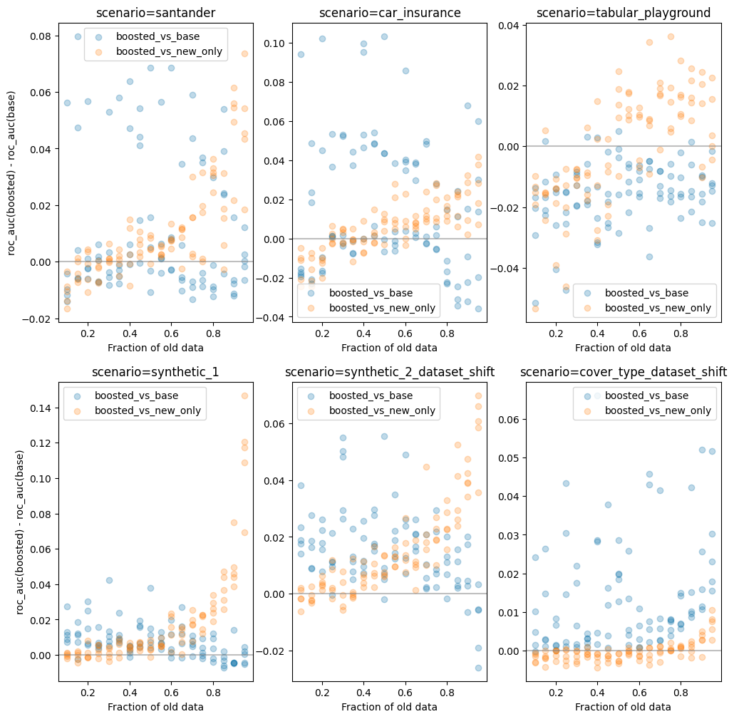
The x-axis of the graph consists of different sizes of the old dataset, ranging from 10% to 95%. The Y-axis represents the delta in model
performance (roc_auc) between the boosted model and the two baselines - training on the full dataset (blue) and training on new data only (orange).</p>
<p>Different dots at the same x-value correspond to different (randomized) choices of which columns should be deleted.</p>
<p>There is of course a wide range of performance, as one might expect. If randomly nullifying columns deletes important model features then we expect
performance to go down significantly, giving dataset boosting a greater opportunity to improve things. However if the randomly deleted columns are
simply noise we expect it to be harmless to baseline model performance and dataset boosting will just add further noise.</p>
<p>The pattern that can be seen in most of the graphs is an asymmetric benefit to using this new boosting scheme. When boosting improves performance,
it does so by a large margin. When it hinders performance it's mostly by a much smaller margin.</p>
<p>The only exception here is <code>tabular_playground</code> where it underperfors in all cases. It is interesting to note that on this dataset - unlike all the
others I'm using - logistic regression performs as well as gradient boosting. It is fairly <a href="https://stats.stackexchange.com/questions/186966/gradient-boosting-for-linear-regression-why-does-it-not-work/186974">easy to prove</a> that when a linear model works there is no advantage to boosting, so this should not
be surprising.</p>
<table>
<thead>
<tr>
<th style="text-align: left;">scenario</th>
<th style="text-align: right;">win_base</th>
<th style="text-align: right;">win_new_only</th>
<th style="text-align: right;">delta_base</th>
<th style="text-align: right;">delta_new_only</th>
<th style="text-align: right;">boosted_regret</th>
<th style="text-align: right;">base_regret</th>
<th style="text-align: right;">new_only_regret</th>
</tr>
</thead>
<tbody>
<tr>
<td style="text-align: left;">car_insurance</td>
<td style="text-align: right;">0.600</td>
<td style="text-align: right;">0.633</td>
<td style="text-align: right;">0.016</td>
<td style="text-align: right;">0.006</td>
<td style="text-align: right;">0.011</td>
<td style="text-align: right;">0.028</td>
<td style="text-align: right;">0.017</td>
</tr>
<tr>
<td style="text-align: left;">cover_type_dataset_shift</td>
<td style="text-align: right;">0.989</td>
<td style="text-align: right;">0.378</td>
<td style="text-align: right;">0.014</td>
<td style="text-align: right;">-0.000</td>
<td style="text-align: right;">0.003</td>
<td style="text-align: right;">0.016</td>
<td style="text-align: right;">0.003</td>
</tr>
<tr>
<td style="text-align: left;">santander</td>
<td style="text-align: right;">0.500</td>
<td style="text-align: right;">0.744</td>
<td style="text-align: right;">0.011</td>
<td style="text-align: right;">0.010</td>
<td style="text-align: right;">0.008</td>
<td style="text-align: right;">0.019</td>
<td style="text-align: right;">0.018</td>
</tr>
<tr>
<td style="text-align: left;">synthetic_1</td>
<td style="text-align: right;">0.789</td>
<td style="text-align: right;">0.856</td>
<td style="text-align: right;">0.008</td>
<td style="text-align: right;">0.018</td>
<td style="text-align: right;">0.007</td>
<td style="text-align: right;">0.014</td>
<td style="text-align: right;">0.024</td>
</tr>
<tr>
<td style="text-align: left;">synthetic_2_dataset_shift</td>
<td style="text-align: right;">0.911</td>
<td style="text-align: right;">0.844</td>
<td style="text-align: right;">0.015</td>
<td style="text-align: right;">0.018</td>
<td style="text-align: right;">0.033</td>
</tr>
<tr>
<td style="text-align: left;">tabular_playground</td>
<td style="text-align: right;">0.056</td>
<td style="text-align: right;">0.522</td>
<td style="text-align: right;">-0.015</td>
<td style="text-align: right;">0.000</td>
<td style="text-align: right;">0.017</td>
<td style="text-align: right;">0.001</td>
<td style="text-align: right;">0.017</td>
</tr>
</tbody>
</table>
<p>The columns <code>win_base</code> and <code>win_new_only</code> represent the fraction of times when my dataset boosting scheme outperforms training the model on either
the full dataset (<code>win_base) or the new rows only (</code>win_new_only<code>). The</code>delta_base<code>/</code>delta_new_only<code>columns represent the average lift.
Finally, the</code>?_regret` columns represent the difference in performance between a model trained on the full dataset (i.e. without dropping any data)
and the model trained on the censored dataset. This is averaged across all simulations.</p>
<h2>Relevance of the censored features</h2>
<p>A natural question arises - how does the benefit of dataset boosting relate to the importance of the features that are missing in the old data?</p>
<p><strong>The meaning of importance:</strong> It is important to clarify that by "importance", I mean the importance of the features to a model trained
on <em>full uncensored data</em>. I have evaluated this by training a model on the full data (the same ones used to compute regret) and then using
<code>sklearn.inspection.permutation_importance</code> to compute the importance of each feature.</p>
<p>Some reasoning:</p>
<ol>
<li>As the importance of the censored features increases we would expect the benefit of boosting relative to training on the full dataset to increase.
This is because in the full model (trained on all data), the fraction of the dataset which contains the high importance features is very low. Whereas
in the boosted model, we have constructed a model so that these features are treated as if they are fully available, which they are.</li>
<li>As the importance of uncensored features decreases, we would expect the base model (trained on censored data only) to provide little/no useful information.
 hus, in this situation, the model trained on new data only become the "best possible" model and the dataset boosting scheme will simply be adding noise.</li>
</ol>
<p>To test this theory I ran a similar simulation to what is described above. However this time I kept the fraction of the dataset which is old constant
(at 85%) while varying the number of features which were dropped.</p>
<p><img alt="Graph of performance" src="https://www.chrisstucchio.com/blog_media/2022/boosting_for_dataset_changes/deleted_importance.png"></p>
<p>
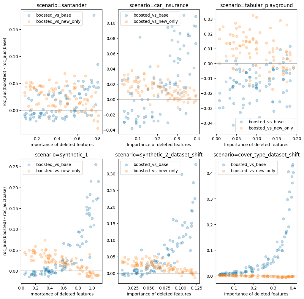
As can be seen, on most datasets for which boosting is helpful, the pattern I speculated about above does seem to hold out.</p>
<h1>Conclusion</h1>
<p>In many of the simple examples I've tested it with here, this boosting scheme seems to be a significant improvement over the most obvious alternative approaches.</p>
<p>Dataset boosting is generally beneficial when:</p>
<ol>
<li>The old data comprises a large fraction (80% or more) of the dataset.</li>
<li>The new data is not large enough to train an accurate model by restricting solely to the new data.</li>
<li>The features present in the old data and the features missing from the old data both have significant importance.</li>
</ol>
<p>It is not beneficial in other cases and mostly seems to add noise, diminishing accuracy.</p>
<p>This shouldn't be very surprising since the theoretical justification and practical applicability of boosting has been known for a long time. But
nevertheless, I've not seen this approach used to address issues related to <em>dataset completeness</em>, and I'm hoping a kind reader might point me to a
body of literature addressing this or persuade someone to research this in greater generality.</p>
<h2>Related</h2>
<ul>
<li><a href="https://www.chrisstucchio.com/blog_media/2022/boosting_for_dataset_changes/2002.11982.pdf">Adapted Tree Boosting for Transfer Learning</a>, some Alipay guys using a similar idea for a somewhat different purpose.</li>
<li><a href="https://www.chrisstucchio.com/blog_media/2022/boosting_for_dataset_changes/samme.pdf">Multiclass adaboost</a> original paper on the topic.</li>
</ul>
<script type="text/javascript">if (!document.getElementById('mathjaxscript_pelican_#%@#$@#')) {
    var align = "center",
        indent = "0em",
        linebreak = "false";

    if (false) {
        align = (screen.width < 768) ? "left" : align;
        indent = (screen.width < 768) ? "0em" : indent;
        linebreak = (screen.width < 768) ? 'true' : linebreak;
    }

    var mathjaxscript = document.createElement('script');
    mathjaxscript.id = 'mathjaxscript_pelican_#%@#$@#';
    mathjaxscript.type = 'text/javascript';
    mathjaxscript.src = 'https://cdnjs.cloudflare.com/ajax/libs/mathjax/2.7.3/latest.js?config=TeX-AMS-MML_HTMLorMML';

    var configscript = document.createElement('script');
    configscript.type = 'text/x-mathjax-config';
    configscript[(window.opera ? "innerHTML" : "text")] =
        "MathJax.Hub.Config({" +
        "    config: ['MMLorHTML.js']," +
        "    TeX: { extensions: ['AMSmath.js','AMSsymbols.js','noErrors.js','noUndefined.js'], equationNumbers: { autoNumber: 'none' } }," +
        "    jax: ['input/TeX','input/MathML','output/HTML-CSS']," +
        "    extensions: ['tex2jax.js','mml2jax.js','MathMenu.js','MathZoom.js']," +
        "    displayAlign: '"+ align +"'," +
        "    displayIndent: '"+ indent +"'," +
        "    showMathMenu: true," +
        "    messageStyle: 'normal'," +
        "    tex2jax: { " +
        "        inlineMath: [ ['\\\\(','\\\\)'] ], " +
        "        displayMath: [ ['$$','$$'] ]," +
        "        processEscapes: true," +
        "        preview: 'TeX'," +
        "    }, " +
        "    'HTML-CSS': { " +
        "        availableFonts: ['STIX', 'TeX']," +
        "        preferredFont: 'STIX'," +
        "        styles: { '.MathJax_Display, .MathJax .mo, .MathJax .mi, .MathJax .mn': {color: 'inherit ! important'} }," +
        "        linebreaks: { automatic: "+ linebreak +", width: '90% container' }," +
        "    }, " +
        "}); " +
        "if ('default' !== 'default') {" +
            "MathJax.Hub.Register.StartupHook('HTML-CSS Jax Ready',function () {" +
                "var VARIANT = MathJax.OutputJax['HTML-CSS'].FONTDATA.VARIANT;" +
                "VARIANT['normal'].fonts.unshift('MathJax_default');" +
                "VARIANT['bold'].fonts.unshift('MathJax_default-bold');" +
                "VARIANT['italic'].fonts.unshift('MathJax_default-italic');" +
                "VARIANT['-tex-mathit'].fonts.unshift('MathJax_default-italic');" +
            "});" +
            "MathJax.Hub.Register.StartupHook('SVG Jax Ready',function () {" +
                "var VARIANT = MathJax.OutputJax.SVG.FONTDATA.VARIANT;" +
                "VARIANT['normal'].fonts.unshift('MathJax_default');" +
                "VARIANT['bold'].fonts.unshift('MathJax_default-bold');" +
                "VARIANT['italic'].fonts.unshift('MathJax_default-italic');" +
                "VARIANT['-tex-mathit'].fonts.unshift('MathJax_default-italic');" +
            "});" +
        "}";

    (document.body || document.getElementsByTagName('head')[0]).appendChild(configscript);
    (document.body || document.getElementsByTagName('head')[0]).appendChild(mathjaxscript);
}
</script>
              ]]>
            </content>
        </entry>
        <entry>
            <title type="html">Calibrating a classifier when the base rate changes</title>
            <author><name>Chris Stucchio</name></author>
            <link href="https://www.chrisstucchio.com/blog/2020/calibrated_classifier_base_rates.html?utm_medium=rss&amp;utm_source=rss&amp;utm_campaign=rss"/>
            <updated>2020-07-07T08:30:00+02:00Z</updated>
            <published>2020-07-07T08:30:00+02:00Z</published>
            <id>https://www.chrisstucchio.com/blog/2020/calibrated_classifier_base_rates.html</id>

            <content type="html">
              <![CDATA[
                (If mathematical formulas are not showing up here, <a href="https://www.chrisstucchio.com/blog/2020/calibrated_classifier_base_rates.html?utm_medium=rss&amp;utm_source=rss&amp;utm_campaign=rss">please read this on the web.</a>.)
                <p>In a previous job, I built a machine learning system to detect financial fraud. Fraud was a big problem at the time - for simplicity of having nice round numbers, suppose 10% of attempted transactions were fraudulent. My machine learning system worked great - as a further set of made-up round numbers, lets describe it as having a precision and recall of 50% each. All this resulted in a fantastic bite taken out of the fraud problem.</p>
<p>It worked so well that fraud dropped by well over 50% - because of the effort involved in getting past the system, fraudsters just gave up and stopped trying to scam us.</p>
<p>Suddenly the system's performance tanked - recall stayed at 50% but precision dropped to 8%! After some diagnosis, I discovered the cause was the following - all the fraudsters had gone away. For every fraud attempt, the system had a 50% chance of flagging it. For every non-fraudulent transaction, the system had a 5.5% chance of flagging it.</p>
<p>Early on, fraud attempts made up 10% of our transactions. Thus, for every 1000 transactions, we would flag 50 of the 100 fraudulent transactions and 50 of the 900 good transactions. This means that for every 10 flags, 5 are correct - hence a precision of 50%.</p>
<p>Once the fraudsters fucked off, fraud attempts dropped to perhaps 1% of our transactions. For every 1000 transactions, only 10 were fraudulent. We would flag 5 of them, along with 5.5% x 990 legitimate transactions = 54 transactions. The net result is that only 5 of the 59 transactions we flagged as fraudulent actually were, for a precision of 8%.</p>
<p>This phenomenon is called <strong>label shift</strong>. The problem with label shift is that the base rate for the target class changes with time and this significantly affects the precision of the classifier.</p>
<div class="section" id="typical-characteristics-of-the-problem">
<h2>Typical characteristics of the problem</h2>
<p>In general, the following are characteristics of the problem that I'm generally interested in:</p>
<ol class="arabic simple">
<li><span class="math">\(N\)</span> not too large - potentially under 100k.</li>
<li><span class="math">\(\alpha\)</span> in the ballpark of 0.1% to 5%.</li>
</ol>
<p>These kinds of problems are typical in security, fraud prevention, medicine, and other situations of attempting to detect harmful anomalous behavior.</p>
<div class="section" id="precision-risk-thresholds-and-loss-functions">
<h3>Precision, Risk Thresholds and Loss Functions</h3>
<p>For most classifiers the ultimate goal is to make a decision. The decision is taken in order to minimize some loss function which represents the real world cost of making a mistake.</p>
<p>Consider as an example a clasifier <span class="math">\(f: \mathbb{R}^K \rightarrow \mathbb{R}\)</span> used to predict a disease. Let us define <span class="math">\(\vec{x} \in \mathbb{R}^K\)</span> to be our feature vector, <span class="math">\(z \in [0,1]\)</span> to be our risk score and <span class="math">\(y \in 0,1\)</span> whether or not the patient actually has the disease.</p>
<p>A loss function might represent the loss in <a class="reference external" href="https://en.wikipedia.org/wiki/Quality-adjusted_life_year">QUALYs</a> from making an error. Concretely, suppose that a failure to diagnose a disease results in the immediate death of the patient - this is a loss of <code>78 - patient's age</code> QUALYs. On the flip side, treatment is also risky - perhaps 5% of patients are allergic and also die instantly. This is a loss of <code>5% x (78 - patient's age)</code> <a class="footnote-reference" href="#lifeexpectancycalc" id="footnote-reference-1">[1]</a>. Represented mathematically, our loss function is:</p>
<div class="math">
\begin{equation*}
L(\textrm{treat}; 0) = 0.05
\end{equation*}
</div>
<div class="math">
\begin{equation*}
L(\textrm{treat}; 1) = 0
\end{equation*}
</div>
<div class="math">
\begin{equation*}
L(\textrm{no~treat}; 0) = 0
\end{equation*}
</div>
<div class="math">
\begin{equation*}
L(\textrm{no~treat}; 1) = 1
\end{equation*}
</div>
<p>Let us also suppose that we have a calibrated risk score, i.e. a monotonically increasing function <span class="math">\(c: [0,1]-&gt;[0,1]\)</span> with the property that <span class="math">\(c(z)=P(y=1|z)\)</span>. For a given patient, the expected loss from treatment is therefore:</p>
<div class="math">
\begin{equation*}
E[L(\textrm{treat}; y)] = (1-c(z)) \cdot 0.05
\end{equation*}
</div>
<p>while the loss from non-treatment is:</p>
<div class="math">
\begin{equation*}
E[L(\textrm{no~treat}; y)] = c(z) \cdot 1 = c(z)
\end{equation*}
</div>
<p>The expected loss from treatment exceeds the expected loss from non-treatment when <span class="math">\(c(z) &gt; 0.05/1.05 \approx 0.0526\)</span>, so the optimal decision rule is to treat every patient with a (calibrated) risk score larger than 0.0526 while letting the others go untreated.</p>
</div>
</div>
<div class="section" id="the-effect-of-label-shift-on-calibration">
<h2>The effect of label shift on calibration</h2>
<p>Let's study this from the perspective of score distributions. Suppose that <span class="math">\(f_0(z)\)</span> is the pdf of the distribution <span class="math">\(z | y=0\)</span> and <span class="math">\(f_1(z)\)</span> is the pdf of the distribution <span class="math">\(z | y=1\)</span>. For simplicity, assume these distributions are monotonic.</p>
<p>Suppose now that the base rate is <span class="math">\(P(y=1)=\alpha\)</span>. In this framework, a label shift can be represented simply as a change in <span class="math">\(\alpha\)</span>.</p>
<p>It is straightforward to calculate the calibration curve (as a function <span class="math">\(\alpha\)</span>) as:</p>
<div class="math">
\begin{equation*}
P(y=1|z,\alpha) = c(z;\alpha) = \frac{ \alpha f_1(z) }{ (1-\alpha)f_0(z) + \alpha f_1(z) }
\end{equation*}
</div>
<p>As is apparent from this formula, a change in <span class="math">\(\alpha\)</span> will result in a change in calibration. The following graph provides an example:</p>
<div class="figure" id="fig-diff-calibration-curves" style="width: 600px">
<img alt="" src="https://www.chrisstucchio.com/blog_media/2020/calibrated_classifier_base_rates/calibration_shift.png" />
<p class="caption">Illustration of calibration curves changing with base rate</p>
</div>
<p>Let's consider the effect of this on decisionmaking. Going back to our disease example above, suppose that at model training/calibration time, <span class="math">\(\alpha=0.01\)</span>. Then a disease outbreak occurs and <span class="math">\(\alpha=0.1\)</span>. The decision rule being used based on the training data (with <span class="math">\(\alpha=0.01\)</span>) says to treat any patient with raw <span class="math">\(z\)</span> score of 0.65 or greater.</p>
<p>But once <span class="math">\(\alpha=0.1\)</span>, the actual infection probability of a person with <span class="math">\(z=0.65\)</span> is nearly 40%. As per the loss function calculation earlier, we want to treat any patient with a 5.26% or greater chance of being sick!</p>
<p>In the literature, when making batch predictions, there's a <a class="reference external" href="https://www.chrisstucchio.com/blog_media/2020/calibrated_classifier_base_rates/Adjusting_the_Outputs_of_a_Classifier_to_New_a_Priori_Probabilities_A_Simple_Procedure__Saerens2002a.pdf">known technique for solving this</a> (see discussion <a class="footnote-reference" href="#saerens" id="footnote-reference-2">[2]</a>). The basic idea is the following. For a set of raw risk scores <span class="math">\(z_i, i=1\ldots N\)</span>, we know they are drawn from the distribution:</p>
<div class="math">
\begin{equation*}
z_i \leftarrow [(1-\alpha)f_0(Z) + \alpha f_1(Z)] dz
\end{equation*}
</div>
<p>Thus, one can estimate <span class="math">\(\alpha\)</span> via the maximum likelihood principle (although the literature describes a slightly different approach <a class="footnote-reference" href="#serensdiff" id="footnote-reference-3">[3]</a>):</p>
<div class="math">
\begin{equation*}
\alpha = \textrm{arg} \max \prod_{i=1}^N \left[(1-\alpha)f_0(z_i) + \alpha f_1(z_i)\right]
\end{equation*}
</div>
<p>Maximizing this is straightforward - take logs, compute <span class="math">\(\frac{\partial L}{\partial \alpha}\)</span>, use <a class="reference external" href="https://docs.scipy.org/doc/scipy/reference/generated/scipy.optimize.minimize.html">scipy.optimize.minimize</a>.</p>
<div class="section" id="what-happens-when-the-distribution-changes">
<h3>What happens when the distribution changes?</h3>
<p>The method described above is strongly sensitive to the assumption that the <em>shape</em> of the distribution of the positive class <span class="math">\(f_1(z)\)</span> does not change, only it's amplitude <span class="math">\(\alpha\)</span>.</p>
<p>However in practice, we often discover that <span class="math">\(f_1(Z)\)</span> changes with time as well. For example, consider again the example of disease prediction - a new strain of a known disease may have a somewhat different symptom distribution in the future than in the past. However it is a reasonable assumption to make that the shape of <span class="math">\(f_0(z)\)</span> remains the same; healthy people do not change their health profile until they become infected.</p>
<p>Thus, the more general situation I'm considering is a mix of label shift/base rate changes, together with small to moderate changes in the distribution of the <em>exceptional class only</em>. By &quot;exceptional class&quot;, I mean &quot;sick&quot; (in disease prediction), &quot;fraud&quot; (in fraud prevention), essentially the uncommon label which corresponds to something anomalous.</p>
<p>In general, it is impossible to solve this problem <a class="footnote-reference" href="#impossibility" id="footnote-reference-4">[5]</a>. However, if we stay away from this degenerate case (see footnote <a class="footnote-reference" href="#impossibility" id="footnote-reference-5">[5]</a>), it's actually quite possible to solve this problem and estimate both the new shape of <span class="math">\(f_1(z)\)</span> and <span class="math">\(\alpha\)</span>. The main restriction is that <span class="math">\(f_1(z)\)</span> is not too different from the old value, but right now I don't have a good characterization of what &quot;not too different&quot; actually means.</p>
</div>
</div>
<div class="section" id="formal-statement-of-the-setup">
<h2>Formal statement of the setup</h2>
<p>In the training phase, we have a labelled data set <span class="math">\((\vec{x}_i, y_i), i=1\ldots N\)</span> on which we can train any sort of model that generates risk scores <span class="math">\(z_i, i=1 \ldots N\)</span>. We will assume that in this data set, the risk scores <span class="math">\(z_i\)</span> are drawn from <span class="math">\(f_0(z)\)</span> if <span class="math">\(y_i=0\)</span> and <span class="math">\(f_1(z)\)</span> if <span class="math">\(y_i=1\)</span>.</p>
<p>In the prediction phase we will consider batch predictions. We receive a new set of <span class="math">\(\vec{x}\)</span> and we can of course use the already trained classifier to generate risk scores <span class="math">\(z_i\)</span>. Our goal is for each data point <span class="math">\(z_i\)</span> to generate a calibrated risk score <span class="math">\(c(z_i) \approx P(y_i=1|z_i)\)</span>.</p>
<p>Without label shift there is a standard approach to this that is implemented in sklearn as <a class="reference external" href="https://scikit-learn.org/stable/modules/generated/sklearn.calibration.CalibratedClassifierCV.html">sklearn.calibration.CalibratedClassifierCV</a>. Typically this involves running isotonic regression on a subset of the training data and the mapping <span class="math">\(c(z)\)</span> is the result of this.</p>
<p>That does not work in this case because <span class="math">\(c(z)\)</span> computed in the training phase will be for the <em>wrong</em> distribution. The figure <a class="reference external" href="fig_diff_calibration_curves">Illustration of calibration curves changing with base rate</a> illustrates this - isotonic calibration may correctly fit the curve <span class="math">\(c(z; \alpha=0.01)\)</span> in the training phase. But if the right curve in the prediction phase is <span class="math">\(c(z; \alpha=0.1)\)</span>, that fit is not actually correct. This blog post aims to address that problem.</p>
</div>
<div class="section" id="my-method">
<h2>My method</h2>
<p>The approach I'm taking is upgrading the maximum likelihood estimation to a max-aposteriori estimation.</p>
<p>I first parameterize the shape of the exceptional label <span class="math">\(f_1(z;\vec{q})\)</span> with <span class="math">\(\vec{q} \in \mathbb{R}^m\)</span>. I then construct a Bayesian prior on it which is clustered near <span class="math">\(f_1(z)\)</span>. It is straightforwardly derived from Bayes rule that x:</p>
<div class="math">
\begin{equation*}
P\left(\alpha, \vec{q} | \{z_i\}_{1}^{N} \right) \propto P\left(\{z_i\}_{1}^{N}|\alpha, \vec{q}\right) P(\alpha, \vec{q}) = P(\alpha, \vec{q}) \prod_{i=1}^N \left[(1-\alpha)f_0(z_i) + \alpha f_1(z_i; \vec{q})\right]
\end{equation*}
</div>
<p>For simplicity I'm taking <span class="math">\(P(\alpha, \vec{q}) = P(\vec{q})\)</span>, a uniform prior on <span class="math">\(\alpha\)</span>.</p>
<p>Once the posterior is computed, we can replace <em>maximum likelihood</em> with <em>max-aposteriori</em> estimation. This provides a plausible point estimate for <span class="math">\((\alpha, \vec{q})\)</span> which we can then use for calibration.</p>
</div>
<div class="section" id="kernel-density-estimation-on-0-1">
<h2>Kernel Density Estimation on [0,1]</h2>
<p>The first step is doing kernel density estimation in 1-dimension in a manner that respects the domain of the function. Gaussian KDE does NOT fit the bill here because the support of a gaussian kernel is <span class="math">\(\mathbb{R}\)</span>, not <span class="math">\([0,1]\)</span>. One approach (which is somewhat technical and I couldn't make performant) is using beta-function KDE instead <a class="footnote-reference" href="#betakde" id="footnote-reference-6">[4]</a>. An additional technical challenge with using traditional KDE approaches on this problem is that whatever approach is taken, it also needs to be fit into a max-likelihood/max-aposteriori type method.</p>
<p>I took a simpler approach and simply used linear splines in a manner that's easy to work with in scipy. Suppose we have node points <span class="math">\(\zeta_0=0, \zeta_1, \ldots, \zeta_m=1\)</span>. Then let us define the distribution <span class="math">\(f_1(z; \vec{q})\)</span> as a normal piecewise linear function:</p>
<div class="math">
\begin{equation*}
f_1(z; \vec{q}) = \frac{z-\zeta_k}{\zeta_{k+1}-\zeta_k} h_{k} +  \frac{\zeta_{k+1} - z}{\zeta_{k+1}-\zeta_k} h_{k+1}
\end{equation*}
</div>
<p>for <span class="math">\(z \in [\zeta_k,\zeta_{k+1}]\)</span> with <span class="math">\(h_i\)</span> defined as</p>
<div class="math">
\begin{equation*}
h_i=e^{q_i} / M(\vec{q}), i=1\ldots N
\end{equation*}
</div>
<div class="math">
\begin{equation*}
h_0=1/M(\vec{q})
\end{equation*}
</div>
<p>and</p>
<div class="math">
\begin{equation*}
M(\vec{q}) = \int_a^b p(x) dx = \sum_{i=1}^N \frac{1}{2} (e^{q_i}+e^{q_{i-1}})(\zeta_i-\zeta_{i-1}).
\end{equation*}
</div>
<p>I chose this parameterization because <code>scipy.optimize.minimize</code> doesn't do constrained optimization very well. With this parameterization, all values <span class="math">\(\vec{q} \in \mathbb{R}^m\)</span> yield a valid probability distribution on <span class="math">\([0,1]\)</span>.</p>
<p>Python code implementing this is available in the linked notebook, implemented as <code>PiecewiseLinearKDE</code>. Calculations of <span class="math">\(\nabla_{\vec{q}} h_i(\vec{q})\)</span> - used in numerical optimization - can also be found in that notebook. Most of it is straightforward.</p>
<p>Fitting a piecewise linear distribution to data is only a few lines of code:</p>
<pre class="code literal-block">
from scipy.optimize import minimize
def objective(q):
    p = PiecewiseLinearKDE(zz, q)
    return -1*np.log(p(z)+reg).sum() / len(z)

def deriv(q):
    p = PiecewiseLinearKDE(zz, q)
    return -1*p.grad_q(z) &#64; (1.0/(p(z)+reg)) / len(z)

result = minimize(objective, jac=deriv, x0=np.zeros(shape=(len(zeta)-1,)), method='tnc', tol=1e-6, options={'maxiter': 10000})
result = PiecewiseLinearKDE(zeta, result.x)
</pre>
<img alt="" src="https://www.chrisstucchio.com/blog_media/2020/calibrated_classifier_base_rates/mle_fit_one_dist.png" />
<p>The result is approximately what one might expect.</p>
<p>One useful coding trick to take away from this is our use of <code>np.interp</code> inside a number of methods of <code>PiecewiseLinearKDE</code>. Since the curve itself is computed as <code>np.interp(x, self.nodes, self.h())</code>, gradients of this w.r.t. <code>q</code> can then then be computed by applying <code>np.interp(x, self.nodes, grad_h)</code> where <code>grad_h</code> is the gradient of <span class="math">\(\vec{h}\)</span> w.r.t. <span class="math">\(\vec{q}\)</span>. This then allows the efficient calculation of gradients of likelihood functions as seen in <code>deriv</code> above, simplifying what might otherwise be index-heavy code.</p>
</div>
<div class="section" id="computing-a-posterior-and-max-aposteriori-estimation">
<h2>Computing a posterior and max-aposteriori estimation</h2>
<p>Defining a prior on a function space - e.g. the space of all probability distributions on [0,1] - is not a simple matter. However, once we've chosen a parameterization for <span class="math">\(f_1(z; \vec{q})\)</span>, it becomes straightforward. Since <span class="math">\(\vec{q} \in \mathbb{R}^m\)</span>, the restriction of any reasonable prior onto this space is absolutely continuous w.r.t. Lebesgue measure, thereby eliminating any theoretical concerns.</p>
<p>The situation we are attempting to model is a small to moderate <em>change</em> in the distribution of <span class="math">\(f_1(z)\)</span>, particularly in regions where <span class="math">\(f_0(z)\)</span> is small. So we will define the (unnormalized) prior to be:</p>
<div class="math">
\begin{equation*}
\textrm{prior}(\vec{q}) \sim \textrm{exp} \left( -\beta \int_0^1 \left[g(f_1(z; \vec{q}) - f_1(z))\right]^p f_0(z) dz \right)
\end{equation*}
</div>
<p>where <span class="math">\(g(x) = \sqrt{1+x^2}-1\)</span> is a basically just a smoothed out (differentiable) version of <span class="math">\(|x|\)</span>. We need a smooth version of <span class="math">\(|x|\)</span> simply because when we do max-aposteriori later, a smooth curve makes numerical minimization easier.</p>
<p>This prior should not be thought of as a principled Bayesian prior, but merely one chosen for convenience and because it regularizes the method. If we ignore the smoothing, this is analogous to a prior that penalizes deviation from <span class="math">\(f_1(z)\)</span> in the <span class="math">\(L^p(f_0(z) dz)\)</span> metric. The measure <span class="math">\(f_0(z) dz\)</span> is used to penalize deviation more in areas where <span class="math">\(f_0(z)\)</span> is large. The parameter <span class="math">\(\beta\)</span> represents the strength of the prior - larger <span class="math">\(\beta\)</span> means that <span class="math">\(f_1(z; \vec{q})\)</span> will remain closer to <span class="math">\(f_1(z)\)</span>.</p>
<p>One important note about the power <span class="math">\(p\)</span>. Because <span class="math">\(g(x) = O(x^2)\)</span> as <span class="math">\(x \rightarrow 0\)</span>, choosing <span class="math">\(p=1\)</span> does NOT actually generate any kind of sparsity penalty, in contrast to using <span class="math">\(|x|^1\)</span>.</p>
<p>The likelihood is (as per the above):</p>
<div class="math">
\begin{equation*}
\textrm{likelihood}(\alpha, \vec{q}) \equiv P(\{z_i\}_{1}^{N}|\alpha, \vec{q}) = \prod_{i=1}^N \left[(1-\alpha)f_0(z_i) + \alpha f_1(z_i; \vec{q})\right]
\end{equation*}
</div>
<p>Computing the log of likelihood times prior (neglecting the normalization term from Bayes rule), we obtain:</p>
<div class="math">
\begin{equation*}
\log[\textrm{prior}(\vec{q})\textrm{likelihood}(\alpha, \vec{q})] = \left( \sum_{i=1}^N \log \left[(1-\alpha)f_0(z_i) + \alpha f_1(z_i; \vec{q})\right] \right)
\end{equation*}
</div>
<div class="math">
\begin{equation*}
- \beta \int_0^1 \left[g(f_1(z; \vec{q}) - f_1(z))\right]^p f_0(z) dz
\end{equation*}
</div>
<p>The gradient of this with respect to <span class="math">\((\alpha, \vec{q})\)</span> is:</p>
<div class="math">
\begin{equation*}
\frac{ \partial \ln(P(\{z_i\}_{1}^{N}|\vec{q},\alpha)}{\partial \alpha} = \sum_{i=1}^N \frac{ f_1(z_i; \vec{q}) - f_0(z_i) }{(1-\alpha)f_0(z_i) + \alpha f_1(z_i; \vec{q}) }
\end{equation*}
</div>
<div class="math">
\begin{equation*}
\nabla_{\vec{q}} \ln(P(\{z_i\}_{1}^{N}|\vec{q},\alpha) = \sum_{i=1}^N \frac{\alpha}{(1-\alpha)f_0(z_i) + \alpha f_1(z_i; \vec{q}) } \nabla_{\vec{q}} f_1(z_i; \vec{q})
\end{equation*}
</div>
<div class="math">
\begin{equation*}
- \beta \int_0^1 p g( f_1(\zeta; \vec{q}) - f_1(\zeta) )^{p-1} \frac{[f_1(\zeta; \vec{q}) - f_1(\zeta)] }{\sqrt{1+[f_1(\zeta; \vec{q}) - f_1(\zeta)]^2}}\left[ \nabla_{\vec{q}} f_1(\zeta;\vec{q}) \right] f_0(\zeta) d\zeta
\end{equation*}
</div>
<p>Using this objective function and gradient, it is straightforward to use <a class="reference external" href="https://docs.scipy.org/doc/scipy/reference/generated/scipy.optimize.minimize.html">scipy.optimize.minimize</a> to simultaneously find both <span class="math">\(\vec{q}\)</span> and <span class="math">\(\alpha\)</span>.</p>
<div class="section" id="examples">
<h3>Examples</h3>
<p><strong>Note:</strong> All of the examples here are computed in this <a class="reference external" href="https://www.chrisstucchio.com/blog_media/2020/calibrated_classifier_base_rates/dynamic_calibration.ipynb">Jupyter notebook</a>. For more specific details on how they were performed, the notebook is the place to look.</p>
<p>Here's an example. I took a distribution of 97.7% negative samples, with a relatively simple prior distribution. I simulated a significant change of shape in the distribution of <span class="math">\(z\)</span> scores of the positive class, which is illustrated in red in the graph below. As can be seen, the approximation (the orange line) is reasonably good. Moreover, we recover <span class="math">\(\alpha\)</span> with reasonable accuracy - the measured <span class="math">\(\alpha\)</span> was 0.0225 while the true <span class="math">\(\alpha\)</span> was 0.0234.</p>
<img alt="" src="https://www.chrisstucchio.com/blog_media/2020/calibrated_classifier_base_rates/fitting_the_curve.png" />
<p>(The histograms in the graph illustrate the actual samples drawn.)</p>
<p>Using the fitted curve to compute calibration seems to work reasonably well, although simple isotonic regression is another way to do it.</p>
<img alt="" src="https://www.chrisstucchio.com/blog_media/2020/calibrated_classifier_base_rates/calibration_in_sample.png" />
<p>The advantage of using this method is on out of sample data with a significantly different distribution of positive cases. I repeated this experiment, but with <span class="math">\(\alpha=0.011\)</span> and a marginally different distribution of positive cases.</p>
<img alt="" src="https://www.chrisstucchio.com/blog_media/2020/calibrated_classifier_base_rates/calibration_out_of_sample.png" />
<p>The dynamically calculated calibration curve (the green) still behaves well, while the isotonic fit calculated <em>for a different</em> <span class="math">\(\alpha\)</span> (unsurprisingly) does not provide good calibration.</p>
<p>Note that recalculating the isotonic fit is not possible, since that requires outcome data which is not yet available.</p>
</div>
</div>
<div class="section" id="estimating-bayes-loss">
<h2>Estimating Bayes loss</h2>
<p>The major use case for this method of calibration is reducing the loss of a decision rule due to model miscalibration. Consider a loss function which penalizes false positives and false negatives. Without loss of generality <a class="footnote-reference" href="#loss-function-form" id="footnote-reference-7">[6]</a>, such a loss function takes this form:</p>
<div class="math">
\begin{equation*}
L(1; 0) = 1/(1-T)
\end{equation*}
</div>
<div class="math">
\begin{equation*}
L(1; 1) = 0
\end{equation*}
</div>
<div class="math">
\begin{equation*}
L(0; 0) = 0
\end{equation*}
</div>
<div class="math">
\begin{equation*}
L(0; 1) = 1/T
\end{equation*}
</div>
<p>With this loss function, the optimal decision rule is to choose 1 (positive) whenever <span class="math">\(c(z) &gt;= T\)</span>, otherwise choose 0 (negative).</p>
<p>Using the same example as above, we can compute the result of applying this decision rule using either isotonic calibration (static) or our dynamic rule to the test set. For almost every choice of threshold <span class="math">\(T\)</span>, the loss is significantly lower when using the dynamic calibration.</p>
<img alt="" src="https://www.chrisstucchio.com/blog_media/2020/calibrated_classifier_base_rates/bayes_loss.png" />
</div>
<div class="section" id="other-metrics">
<h2>Other metrics</h2>
<p>A method such as this should NOT be expected to improve <a class="reference external" href="https://en.wikipedia.org/wiki/Receiver_operating_characteristic">ROC_AUC</a>, and in fact in empirical tests this method does not. This is because ROC_AUC is based primarily on ordering of risk scores, and our calibration rule does not change the ordering.</p>
<p>The <a class="reference external" href="https://en.wikipedia.org/wiki/Brier_score">Brier Score</a> - an explicit metric of calibration - does tend to increase with this method. This is of course completely expected. In my experiments, this method is less effective at generating a low Brier score than Isotonic calibration at least until either <span class="math">\(\alpha\)</span> or <span class="math">\(\vec{q}\)</span> changes.</p>
<p>The <a class="reference external" href="https://scikit-learn.org/stable/modules/generated/sklearn.metrics.average_precision_score.html">average precision score</a> also tends to increase over <em>multiple batches</em> with different <span class="math">\(\alpha, \vec{q}\)</span>.</p>
</div>
<div class="section" id="comparison-to-more-standard-label-shift-methods">
<h2>Comparison to more standard label shift methods</h2>
<p>Another approach (the approach of papers linked in footnote <a class="footnote-reference" href="#saerens" id="footnote-reference-8">[2]</a>) is to simply fit <span class="math">\(\alpha\)</span> and do not allow <span class="math">\(f_1(z)\)</span> to change.</p>
<p>In experiments, I've noticed that fitting <span class="math">\(\alpha\)</span> without allowing <span class="math">\(f_1(z)\)</span> to change generally produces a more accurate estimate of <span class="math">\(\alpha\)</span>, even in situations where the true distribution differs significantly from <span class="math">\(f_1(z)\)</span>.</p>
<p>However, in spite of a more accurate estimate of <span class="math">\(\alpha\)</span>, the resulting calibration curves from fitting only <span class="math">\(\alpha\)</span> do not tend to be as accurate. The curve that comes from fitting <span class="math">\(\alpha, \vec{q}\)</span> is more accurate than the fit of <span class="math">\(\alpha\)</span> alone:</p>
<img alt="" src="https://www.chrisstucchio.com/blog_media/2020/calibrated_classifier_base_rates/compare_to_mlls.png" />
<div class="section" id="future-work">
<h3>Future work</h3>
<p>At this stage I do not consider this method in any sense &quot;production ready&quot;. I do not have a great grasp on the conditions when this method works or fails. I've also observed that very frequently, <code>scipy.optimize.minimize</code> fails to converge, yet returns a useful result anyway. Most likely I'm looking for too high a tolerance.</p>
<p>I've also tried a couple of other ways to parameterize the probability distributions and the method seems quite sensitive to them. For example, I included an unnecessary parameter in an earlier variation - <span class="math">\(h_0=e^{q_0}/M(\vec{q})\)</span> - and this completely caused the method to fail to converge. I'm not entirely sure why.</p>
<p>There is a corresponding <a class="reference external" href="https://www.chrisstucchio.com/blog_media/2020/calibrated_classifier_base_rates/dynamic_calibration.ipynb">Jupyter notebook</a> which has the code to do this this. If anyone finds this useful and is able to move it forward, please let me know! As a warning, playing around with the code in the notebook will make the warts of the method fairly visible - e.g. once in a while, a cell will fail to converge, or just converge to something a bit weird.</p>
<p>However, overall I am encouraged by this. I believe it's a promising approach to dynamically adjusting calibration curves and better using prediction models in a context when the distribution of the positive class is highly variable.</p>
</div>
</div>
<div class="section" id="active-learning">
<h2>Active learning</h2>
<p>As one additional note, I'll mention that I have some work (which I'll write about soon) suggesting that if we can request labels for a subset of the data points, we can do reasonably efficient active learning of calibration curves. This appears to significantly improve accuracy and reduce the number of samples needed.</p>
<p class="rubric"><strong>Notes</strong></p>
<table class="docutils footnote" frame="void" id="lifeexpectancycalc" rules="none">
<colgroup><col class="label" /><col /></colgroup>
<tbody valign="top">
<tr><td class="label"><a class="fn-backref" href="#footnote-reference-1">[1]</a></td><td>In reality 78 should be replaced with life expectancy <em>at the time of diagnosis</em>, which is typically larger than the mean population life expectancy. This is a technical detail irrelevant for this post.</td></tr>
</tbody>
</table>
<table class="docutils footnote" frame="void" id="saerens" rules="none">
<colgroup><col class="label" /><col /></colgroup>
<tbody valign="top">
<tr><td class="label">[2]</td><td><em>(<a class="fn-backref" href="#footnote-reference-2">1</a>, <a class="fn-backref" href="#footnote-reference-8">2</a>, <a class="fn-backref" href="#footnote-reference-9">3</a>)</em> <a class="reference external" href="https://www.chrisstucchio.com/blog_media/2020/calibrated_classifier_base_rates/Adjusting_the_Outputs_of_a_Classifier_to_New_a_Priori_Probabilities_A_Simple_Procedure__Saerens2002a.pdf">Adjusting the Outputs of a Classifier to New a Priori Probabilities: A Simple Procedure</a>, by Marco Saerens, Patrice Latinne &amp; Christine Decaestecker. Another useful paper is <a class="reference external" href="https://www.chrisstucchio.com/blog_media/2020/calibrated_classifier_base_rates/EM_with_Bias_Corrected_Calibration_is_Hard_To_Beat_at_Label_Shift_Adaptation__1901.06852v4.pdf">EM with Bias-Corrected Calibration is Hard-To-Beat at Label Shift Adaptation</a> which compares the maximum likelihood method with other more complex methods and finds it's generally competitive. This <a class="reference external" href="https://www.chrisstucchio.com/blog_media/2020/calibrated_classifier_base_ratesA_Unified_View_of_Label_Shift_Estimation__2003.07554v1.pdf">paper</a> also suggests max likelihood type methods are usually the best.</td></tr>
</tbody>
</table>
<table class="docutils footnote" frame="void" id="serensdiff" rules="none">
<colgroup><col class="label" /><col /></colgroup>
<tbody valign="top">
<tr><td class="label"><a class="fn-backref" href="#footnote-reference-3">[3]</a></td><td>The approach taken in the papers cited in <a class="footnote-reference" href="#saerens" id="footnote-reference-9">[2]</a> are a bit different - they do expectation maximization and actually generate parameters representing outcome variables, requiring use of expectation maximization. The approach I'm describing just represents likelihoods of z-scores and ignores outcomes. But in principle these approaches are quite similar, and in testing the version I use tends to be a bit simpler and still works.</td></tr>
</tbody>
</table>
<table class="docutils footnote" frame="void" id="betakde" rules="none">
<colgroup><col class="label" /><col /></colgroup>
<tbody valign="top">
<tr><td class="label"><a class="fn-backref" href="#footnote-reference-6">[4]</a></td><td><a class="reference external" href="https://www.chrisstucchio.com/blog_media/2020/calibrated_classifier_base_rates/Adaptive_Estimation_of_a_Density_Function_Using_Beta_Kernels__BK-2014.pdf">Adaptive Estimation of a Density Function Using Beta Kernels</a> by Karine Bertin and Nicolas Klutchnikoff.</td></tr>
</tbody>
</table>
<table class="docutils footnote" frame="void" id="impossibility" rules="none">
<colgroup><col class="label" /><col /></colgroup>
<tbody valign="top">
<tr><td class="label">[5]</td><td><em>(<a class="fn-backref" href="#footnote-reference-4">1</a>, <a class="fn-backref" href="#footnote-reference-5">2</a>)</em> Suppose that the distribution <span class="math">\(f_1(z)\)</span> changes so that <span class="math">\(f_1(z)=f_0(z)\)</span>. Then for all <span class="math">\(\alpha_0, \alpha_1 \in [0,1]\)</span>, <span class="math">\([(1-\alpha_0)f_0(Z) + \alpha_0 f_1(Z)] \equiv [(1-\alpha_1)f_0(Z) + \alpha_1 f_1(Z)]\)</span> and therefore it is impossible to distinguish between different values of <span class="math">\(\alpha\)</span> from the distribution of <span class="math">\(z\)</span> alone.</td></tr>
</tbody>
</table>
<table class="docutils footnote" frame="void" id="loss-function-form" rules="none">
<colgroup><col class="label" /><col /></colgroup>
<tbody valign="top">
<tr><td class="label"><a class="fn-backref" href="#footnote-reference-7">[6]</a></td><td>Suppose we had an arbitrary loss function with a false positive cost of <span class="math">\(A\)</span> and a false negative cost of <span class="math">\(B\)</span>. Then define <span class="math">\(T=(A/B)/(1+A/B)\)</span> and <span class="math">\(C=BT\)</span>. This is equivalent to a loss function with penalties <span class="math">\(C/(1-T)\)</span> for false positives and <span class="math">\(C/T\)</span> for false negatives, which differs from our choice of loss function only by a multiplicative constant <span class="math">\(C\)</span>.</td></tr>
</tbody>
</table>
</div>
<script type='text/javascript'>if (!document.getElementById('mathjaxscript_pelican_#%@#$@#')) {
    var align = "center",
        indent = "0em",
        linebreak = "false";

    if (false) {
        align = (screen.width < 768) ? "left" : align;
        indent = (screen.width < 768) ? "0em" : indent;
        linebreak = (screen.width < 768) ? 'true' : linebreak;
    }

    var mathjaxscript = document.createElement('script');
    mathjaxscript.id = 'mathjaxscript_pelican_#%@#$@#';
    mathjaxscript.type = 'text/javascript';
    mathjaxscript.src = 'https://cdnjs.cloudflare.com/ajax/libs/mathjax/2.7.3/latest.js?config=TeX-AMS-MML_HTMLorMML';

    var configscript = document.createElement('script');
    configscript.type = 'text/x-mathjax-config';
    configscript[(window.opera ? "innerHTML" : "text")] =
        "MathJax.Hub.Config({" +
        "    config: ['MMLorHTML.js']," +
        "    TeX: { extensions: ['AMSmath.js','AMSsymbols.js','noErrors.js','noUndefined.js'], equationNumbers: { autoNumber: 'none' } }," +
        "    jax: ['input/TeX','input/MathML','output/HTML-CSS']," +
        "    extensions: ['tex2jax.js','mml2jax.js','MathMenu.js','MathZoom.js']," +
        "    displayAlign: '"+ align +"'," +
        "    displayIndent: '"+ indent +"'," +
        "    showMathMenu: true," +
        "    messageStyle: 'normal'," +
        "    tex2jax: { " +
        "        inlineMath: [ ['\\\\(','\\\\)'] ], " +
        "        displayMath: [ ['$$','$$'] ]," +
        "        processEscapes: true," +
        "        preview: 'TeX'," +
        "    }, " +
        "    'HTML-CSS': { " +
        "        availableFonts: ['STIX', 'TeX']," +
        "        preferredFont: 'STIX'," +
        "        styles: { '.MathJax_Display, .MathJax .mo, .MathJax .mi, .MathJax .mn': {color: 'inherit ! important'} }," +
        "        linebreaks: { automatic: "+ linebreak +", width: '90% container' }," +
        "    }, " +
        "}); " +
        "if ('default' !== 'default') {" +
            "MathJax.Hub.Register.StartupHook('HTML-CSS Jax Ready',function () {" +
                "var VARIANT = MathJax.OutputJax['HTML-CSS'].FONTDATA.VARIANT;" +
                "VARIANT['normal'].fonts.unshift('MathJax_default');" +
                "VARIANT['bold'].fonts.unshift('MathJax_default-bold');" +
                "VARIANT['italic'].fonts.unshift('MathJax_default-italic');" +
                "VARIANT['-tex-mathit'].fonts.unshift('MathJax_default-italic');" +
            "});" +
            "MathJax.Hub.Register.StartupHook('SVG Jax Ready',function () {" +
                "var VARIANT = MathJax.OutputJax.SVG.FONTDATA.VARIANT;" +
                "VARIANT['normal'].fonts.unshift('MathJax_default');" +
                "VARIANT['bold'].fonts.unshift('MathJax_default-bold');" +
                "VARIANT['italic'].fonts.unshift('MathJax_default-italic');" +
                "VARIANT['-tex-mathit'].fonts.unshift('MathJax_default-italic');" +
            "});" +
        "}";

    (document.body || document.getElementsByTagName('head')[0]).appendChild(configscript);
    (document.body || document.getElementsByTagName('head')[0]).appendChild(mathjaxscript);
}
</script>
              ]]>
            </content>
        </entry>
        <entry>
            <title type="html">Shareholder Short-Termism Theory has Died of COVID-19</title>
            <author><name>Chris Stucchio</name></author>
            <link href="https://www.chrisstucchio.com/blog/2020/coronavirus_killed_shareholder_short_termism.html?utm_medium=rss&amp;utm_source=rss&amp;utm_campaign=rss"/>
            <updated>2020-06-17T08:30:00+02:00Z</updated>
            <published>2020-06-17T08:30:00+02:00Z</published>
            <id>https://www.chrisstucchio.com/blog/2020/coronavirus_killed_shareholder_short_termism.html</id>

            <content type="html">
              <![CDATA[
                (If mathematical formulas are not showing up here, <a href="https://www.chrisstucchio.com/blog/2020/coronavirus_killed_shareholder_short_termism.html?utm_medium=rss&amp;utm_source=rss&amp;utm_campaign=rss">please read this on the web.</a>.)
                <p>It's become a popular meme that &quot;shareholders only care about the next quarter&quot;. Lots of people make arguments like this - for example, <a class="reference external" href="https://www.wsj.com/articles/short-termism-is-harming-the-economy-1528336801">Jamie Dimon and Warren Buffet</a>. As the meme goes, shareholders only care about the next quarter of earnings, and CEOs make decisions accordingly - sacrificing long term profitability to meet quarterly expectations.</p>
<p>But is this meme true?</p>
<p>Coronavirus gives us a great empirical test of this theory.</p>
<div class="section" id="formalizing-the-theory">
<h2>Formalizing the theory</h2>
<p>The first step in answering this question is to formalize the theory. The most straightforward way I can think of to do this is through the lens of <a class="reference external" href="https://www.investopedia.com/terms/n/npv.asp">net present value</a>, albeit with a modified discount rate.</p>
<p>This framework says that the value of any cash generating asset is given by:</p>
<div class="math">
\begin{equation*}
V = \sum_{t=1}^\infty R_t d_t
\end{equation*}
</div>
<p>In this sum, <span class="math">\(R_t\)</span> is the cash flow in time period <span class="math">\(t\)</span> and <span class="math">\(d_t\)</span> is the <em>discount factor</em> of time <span class="math">\(t\)</span>.</p>
<p>Here's a fairly simple example - a US treasury bill guaranteed to pay a $100 coupon for 3 periods and then to pay a final $10,000 in the 4'th. In tabular form:</p>
<table border="1" class="docutils">
<colgroup>
<col width="67%" />
<col width="33%" />
</colgroup>
<thead valign="bottom">
<tr><th class="head">date</th>
<th class="head">R</th>
</tr>
</thead>
<tbody valign="top">
<tr><td>2020-06-30</td>
<td>100</td>
</tr>
<tr><td>2020-09-30</td>
<td>100</td>
</tr>
<tr><td>2020-12-31</td>
<td>100</td>
</tr>
<tr><td>2021-03-31</td>
<td>10000</td>
</tr>
</tbody>
</table>
<p>To complete the calculation, we need to time discount each cash payment. This is typically done by taking the risk free interest rate - say 5% - and applying that to each time period. For example:</p>
<table border="1" class="docutils">
<colgroup>
<col width="38%" />
<col width="19%" />
<col width="15%" />
<col width="27%" />
</colgroup>
<thead valign="bottom">
<tr><th class="head">date</th>
<th class="head">R</th>
<th class="head">d</th>
<th class="head">R*d</th>
</tr>
</thead>
<tbody valign="top">
<tr><td>2020-06-30</td>
<td>100</td>
<td>1.00</td>
<td>100.00</td>
</tr>
<tr><td>2020-09-30</td>
<td>100</td>
<td>0.99</td>
<td>98.75</td>
</tr>
<tr><td>2020-12-31</td>
<td>100</td>
<td>0.98</td>
<td>97.51</td>
</tr>
<tr><td>2021-03-31</td>
<td>10000</td>
<td>0.96</td>
<td>9631.85</td>
</tr>
</tbody>
</table>
<p>Finally, the value of the bond is the sum of the <code>R*d</code> column, which is $9928.12 in this example.</p>
<div class="section" id="short-termism-in-this-framework">
<h3>Short-Termism in this framework</h3>
<p>In this framework, short-termism can be straightforwardly represented by the <code>d</code> column - specifically, <code>d</code> will rapidly decrease over time. For instance, a very short term valuation of the same bond (a 25% discount rate) might be described as:</p>
<table border="1" class="docutils">
<colgroup>
<col width="38%" />
<col width="19%" />
<col width="15%" />
<col width="27%" />
</colgroup>
<thead valign="bottom">
<tr><th class="head">date</th>
<th class="head">R</th>
<th class="head">d</th>
<th class="head">R*d</th>
</tr>
</thead>
<tbody valign="top">
<tr><td>2020-06-30</td>
<td>100</td>
<td>1.00</td>
<td>100.00</td>
</tr>
<tr><td>2020-09-30</td>
<td>100</td>
<td>0.94</td>
<td>93.90</td>
</tr>
<tr><td>2020-12-31</td>
<td>100</td>
<td>0.88</td>
<td>88.17</td>
</tr>
<tr><td>2021-03-31</td>
<td>10000</td>
<td>0.83</td>
<td>8289.90</td>
</tr>
</tbody>
</table>
<p>which yields a valuation of $8571.97.</p>
<p>Given that Treasury valuations do not look anything like this, we can certainly see that <em>bond</em> investors are not vulnerable to the short-termism that <em>stock</em> investors purportedly suffer from.</p>
<p>The straw man version of &quot;shareholders only care about the next quarter&quot; would mean that <code>d=0</code> for all quarters past the next one.</p>
<p>I will examine this model for mathematical understanding, though I don't think it's a particularly fair thing to do.</p>
</div>
<div class="section" id="modeling-an-uncertain-future">
<h3>Modeling an uncertain future</h3>
<p>Now let us consider a stock rather than a bond - specifically, a pharma company with a single drug in the final phase of clinical trials which end in 1 year.</p>
<p>The cashflow is quite certain for the next 1 year - <code>R[0:4] == 0</code>, i.e. the company loses money to run the clinical trial and pays nothing to shareholders. After 1 year, there are two possible outcomes:</p>
<ol class="arabic simple">
<li>The good outcome. <code>R_good = +1000</code>, the drug works, everyone buys it for 17 years, company is valuable.</li>
<li>The bad outcome. <code>R_bad = 0</code>, the drug does not work, company is worthless.</li>
</ol>
<table border="1" class="docutils">
<colgroup>
<col width="36%" />
<col width="21%" />
<col width="18%" />
<col width="25%" />
</colgroup>
<thead valign="bottom">
<tr><th class="head">date</th>
<th class="head">R_good</th>
<th class="head">R_bad</th>
<th class="head">d</th>
</tr>
</thead>
<tbody valign="top">
<tr><td>2020-06-30</td>
<td>0</td>
<td>0</td>
<td>1.0000</td>
</tr>
<tr><td>2020-09-30</td>
<td>0</td>
<td>0</td>
<td>0.9987</td>
</tr>
<tr><td>2020-12-31</td>
<td>0</td>
<td>0</td>
<td>0.9975</td>
</tr>
<tr><td>2021-03-31</td>
<td>0</td>
<td>0</td>
<td>0.9963</td>
</tr>
<tr><td>2021-06-30</td>
<td>1000</td>
<td>0</td>
<td>0.9950</td>
</tr>
<tr><td>2021-09-30</td>
<td>1000</td>
<td>0</td>
<td>0.9938</td>
</tr>
<tr><td>.</td>
<td>.</td>
<td>.</td>
<td>.</td>
</tr>
<tr><td>2036-06-30</td>
<td>1000</td>
<td>0</td>
<td>0.9231</td>
</tr>
<tr><td>2036-09-30</td>
<td>1000</td>
<td>0</td>
<td>0.9220</td>
</tr>
<tr><td>2036-12-31</td>
<td>1000</td>
<td>0</td>
<td>0.9208</td>
</tr>
<tr><td>2037-03-31</td>
<td>1000</td>
<td>0</td>
<td>0.9197</td>
</tr>
</tbody>
</table>
<p>The company has two eventual valuations (at a long-termist 0.5% discount rate), depending on whether we believe the <code>R_good</code> or <code>R_bad</code> column represents the future - $61,238 in the first case and $0 in the second.</p>
<p>If we assume a 60% chance of the drug getting through clinical trials, then the value of the company would be <code>0.6 * $61238 + 0.4 * 0 = 36742.90</code>.</p>
<p>Note that in the straw man case of <em>literally only the next quarter matters</em>, this company is worth $0 in all possible scenarios - it's first actual profit is 1 year out.</p>
</div>
</div>
<div class="section" id="long-term-investors-appear-short-term">
<h2>Long term investors <em>appear</em> short term</h2>
<p>Lets now consider a long term investor who is evaluating a blue chip, highly stable stock. This stock regularly has earnings of $100. Then one quarter, it misses earnings and only reports $75!</p>
<p>An investor infected by short-termism will significantly cut their evaluation of the company - since <code>d=0</code> for all future periods, the value drops from $100 to $75, a 25% decrease.</p>
<p>Let us now consider a long term investor.</p>
<table border="1" class="docutils">
<colgroup>
<col width="43%" />
<col width="26%" />
<col width="30%" />
</colgroup>
<thead valign="bottom">
<tr><th class="head">date</th>
<th class="head">R</th>
<th class="head">d</th>
</tr>
</thead>
<tbody valign="top">
<tr><td>2020-06-30</td>
<td>75</td>
<td>1.0000</td>
</tr>
<tr><td>2020-09-30</td>
<td>100</td>
<td>0.9987</td>
</tr>
<tr><td>2020-12-31</td>
<td>100</td>
<td>0.9975</td>
</tr>
<tr><td>2021-03-31</td>
<td>100</td>
<td>0.9963</td>
</tr>
<tr><td>2021-06-30</td>
<td>100</td>
<td>0.9950</td>
</tr>
<tr><td>.</td>
<td>.</td>
<td>.</td>
</tr>
</tbody>
</table>
<p>Over 18 years, the value of this revenue stream works out to be $6498. In contrast, had earnings for one quarter not been missed, it would be $6523, a difference of 0.4%. Thus, if there is a drop in share price of significantly more than 0.4%, one might hypothesize that this is due to the market taking a short termist view.</p>
<p>Let us now consider a long term investor who actively tries to think through cause and effect. Earnings decreased, and there must be some reason for it! The question to ask is therefore whether this reduction in a single quarter's earnings will continue into the future. We encounter a situation similar to the pharma stock discussed earlier:</p>
<table border="1" class="docutils">
<colgroup>
<col width="36%" />
<col width="21%" />
<col width="18%" />
<col width="25%" />
</colgroup>
<thead valign="bottom">
<tr><th class="head">date</th>
<th class="head">R_good</th>
<th class="head">R_bad</th>
<th class="head">d</th>
</tr>
</thead>
<tbody valign="top">
<tr><td>2020-06-30</td>
<td>75</td>
<td>75</td>
<td>1.0000</td>
</tr>
<tr><td>2020-09-30</td>
<td>100</td>
<td>75</td>
<td>0.9987</td>
</tr>
<tr><td>.</td>
<td>.</td>
<td>.</td>
<td>.</td>
</tr>
<tr><td>2036-09-30</td>
<td>100</td>
<td>75</td>
<td>0.9220</td>
</tr>
<tr><td>2036-12-31</td>
<td>100</td>
<td>75</td>
<td>0.9208</td>
</tr>
<tr><td>2037-03-31</td>
<td>100</td>
<td>75</td>
<td>0.9197</td>
</tr>
</tbody>
</table>
<p>In the <code>R_bad</code> scenario, the company will only be worth $4892 (a 25% decrease from it's previous value).</p>
<p>If the long term investor believes that there is a 40% chance of this occurring, then the value of the stock decreases to $5855.75, a 10% drop!</p>
<p>Even though the long term investor doesn't care much about a single quarter's earnings, he cares a lot about whether this predicts many more quarters of reduced earnings. This means that even long term investors behave in the manner that others describe as &quot;short-termist&quot;.</p>
<p>As a result, both the short-termism theory and the long-termism theory <em>make very similar predictions</em>. The fact that stock prices move significantly in response to missed earnings estimates is insufficient to distinguish between these two theories.</p>
</div>
<div class="section" id="coronavirus-as-a-natural-experiment">
<h2>Coronavirus as a natural experiment</h2>
<p>Coronavirus provides a great natural experiment to help disambiguate test this theory. A large number of stocks are going to have several quarters of significantly reduced earnings, but there is very little uncertainty as to the reason.</p>
<p>We know that right now people don't go to $SBUX, $MCD or $CMG. This will be a big hit to their earnings. But on the flip side we know exactly why - people haven't suddenly decided they dislike Big Macs, they just don't want to catch coronavirus.</p>
<p>Meanwhile, we're being treated to articles like <a class="reference external" href="https://www.zerohedge.com/markets/great-divide-between-stocks-economy">The Great Divide Between Stocks &amp; The Economy</a> which discuss a significant deviation between stock market performance and <em>short term</em> economic indicators.</p>
<p>One thing is pretty clear: the next couple of quarters of earnings are going to suck. But unlike many earnings misses, we know exactly why. And for most blue chip stocks in the S&amp;P 500, we have great reason to believe that this is strictly temporary, and once coronavirus is dealt with things will go back to normal.</p>
<div class="figure" style="width: 460px">
<img alt="" src="https://www.chrisstucchio.com/blog_media/2020/coronavirus_killed_shareholder_short_termism/spy.png" />
<p class="caption">SPY over time.</p>
</div>
<p>Although SPY is nowadays driven predominantly by technology companies, even brick and mortar companies that are likely to survive the crisis have a similar share price:
This is even true of solid brick and mortar companies such as McDonald's or Starbucks.</p>
<div class="figure" style="width: 460px">
<img alt="" src="https://www.chrisstucchio.com/blog_media/2020/coronavirus_killed_shareholder_short_termism/mcd.png" />
<p class="caption">MCD over time.</p>
</div>
<div class="figure" style="width: 460px">
<img alt="" src="https://www.chrisstucchio.com/blog_media/2020/coronavirus_killed_shareholder_short_termism/sbux.png" />
<p class="caption">SBUX over time.</p>
</div>
<p>If shareholders only care about the next quarter, there is no case to make that $SBUX is worth holding.</p>
<p>However, if shareholders are looking to the long term, then $SBUX and $MCD are pretty solid stocks to hold. If investors have a low discount rate, the impact of the next couple of quarters on LTV is not that big. As long as investors are convinced that there <em>actually is</em> a long term for the company, $SBUX and $MCD remain solid investments. The calculus of a long term investor is exactly as described before:</p>
<table border="1" class="docutils">
<colgroup>
<col width="43%" />
<col width="26%" />
<col width="30%" />
</colgroup>
<thead valign="bottom">
<tr><th class="head">date</th>
<th class="head">R_SBUX</th>
<th class="head">d</th>
</tr>
</thead>
<tbody valign="top">
<tr><td>2020-06-30</td>
<td>50</td>
<td>1.0000</td>
</tr>
<tr><td>2020-09-30</td>
<td>50</td>
<td>0.9987</td>
</tr>
<tr><td>.</td>
<td>.</td>
<td>.</td>
</tr>
<tr><td>2036-09-30</td>
<td>90</td>
<td>0.9220</td>
</tr>
<tr><td>2036-12-31</td>
<td>90</td>
<td>0.9208</td>
</tr>
<tr><td>2037-03-31</td>
<td>90</td>
<td>0.9197</td>
</tr>
</tbody>
</table>
<p>They may not be quite as large after the crisis as before - some locations will certainly close - but overall the revenue stream is likely to continue.</p>
<p>In contrast, other stocks such as $CCL (Carnival Cruise Lines) do not have such a rosy outlook. Unlike $SBUX, $CCL may simply go bankrupt - in that case, shareholders get nothing.</p>
<div class="figure" style="width: 460px">
<img alt="" src="https://www.chrisstucchio.com/blog_media/2020/coronavirus_killed_shareholder_short_termism/ccl.png" />
<p class="caption">CCL over time.</p>
</div>
<p>$CCL is has a very uncertain future. It is likely that it's business will remain solid if it can survive through the crisis - it's August cruises are already fully booked. However, it is not clear that $CCL can actually survive the crisis without going through bankruptcy first. Ships are expensive to store and CCL has financing costs, and it's not clear it can do this without incoming revenue.</p>
<p>This makes it's valuation look a lot more uncertain, with both a good and bad outcome:</p>
<table border="1" class="docutils">
<colgroup>
<col width="36%" />
<col width="21%" />
<col width="18%" />
<col width="25%" />
</colgroup>
<thead valign="bottom">
<tr><th class="head">date</th>
<th class="head">R_good</th>
<th class="head">R_bad</th>
<th class="head">d</th>
</tr>
</thead>
<tbody valign="top">
<tr><td>2020-06-30</td>
<td>0</td>
<td>0</td>
<td>1.0000</td>
</tr>
<tr><td>2020-09-30</td>
<td>0</td>
<td>0</td>
<td>0.9987</td>
</tr>
<tr><td>.</td>
<td>.</td>
<td>.</td>
<td>.</td>
</tr>
<tr><td>2036-09-30</td>
<td>100</td>
<td>0</td>
<td>0.9220</td>
</tr>
<tr><td>2036-12-31</td>
<td>100</td>
<td>0</td>
<td>0.9208</td>
</tr>
<tr><td>2037-03-31</td>
<td>100</td>
<td>0</td>
<td>0.9197</td>
</tr>
</tbody>
</table>
<p>Thus, the stock price of $CCL is remaining low because it is unclear that it ever will come back. There is a high probability assigned to the bad outcome and thus the LTV is low.</p>
<div class="section" id="these-results-are-completely-inconsistent-with-short-termism">
<h3>These results are completely inconsistent with short-termism</h3>
<p>These results are completely inconsistent with a short term &quot;only the next quarter matters&quot; view of the market.</p>
<p>Consider a short term view of $CCL. In the short term view the only quarters which matter are the next few ones, and <em>these quarters are all zero</em> in both the good and bad scenarios. Thus, $CCL is completely worthless for anything besides option value in all possible worlds.</p>
<p>But <em>the same thing is also true for $SBUX and $MCD</em>. For an investor with only short term horizons, $SBUX and $MCD should also be worthless. Yet they have almost completely recovered in value, along with a wide variety of other companies that have a great long term value prop but a terrible short term.</p>
</div>
<div class="section" id="all-about-liquidity-injections">
<h3>All about liquidity injections</h3>
<p>If I had a comment section, I would fully expect someone to talk about how this is all invalid because of the Fed.</p>
<div class="figure" style="width: 500px">
<img alt="" src="https://www.chrisstucchio.com/blog_media/2020/coronavirus_killed_shareholder_short_termism/brrr.jpg" />
</div>
<p>But this betrays a fundamental misunderstanding of accounting. When &quot;money printer go brrr&quot;, the actual mechanism by which this happens is that new debt is issued at favorable terms. Taking out a loan is not earnings so the short term forecast for a company impacted by Coronavirus is unchanged. A short term investor will be completely unmoved by this!</p>
<p>The money printer does have one very important effect - it increases the odds significantly that a company will survive the crisis and have a good <em>long term</em> returns. The next couple of quarters will suck, but the long term value of the company remains.</p>
</div>
</div>
<div class="section" id="the-short-termism-theory-has-died-of-covid">
<h2>The Short-Termism theory has died of COVID</h2>
<p>Coronavirus is a great natural experiment for a lot of things.</p>
<p>One of the most important things we can take away from it is the conclusion that equity markets are fundamentally focused on the long term value of the companies being traded. There are fast responses to problems with next quarter earnings, but these are primarily driven by the fact that problems in the short run tend to be indicative of more fundamental issues.</p>
<p>Now that we have a systematic example where we know that short run problems are strictly short run, we can safely disambiguate between short termism and long termism. The result is very clear; the market is predominantly focused on the long term.</p>
<p><strong>Disclosure:</strong> Long $SBUX, $CCL.</p>
</div>
<script type='text/javascript'>if (!document.getElementById('mathjaxscript_pelican_#%@#$@#')) {
    var align = "center",
        indent = "0em",
        linebreak = "false";

    if (false) {
        align = (screen.width < 768) ? "left" : align;
        indent = (screen.width < 768) ? "0em" : indent;
        linebreak = (screen.width < 768) ? 'true' : linebreak;
    }

    var mathjaxscript = document.createElement('script');
    mathjaxscript.id = 'mathjaxscript_pelican_#%@#$@#';
    mathjaxscript.type = 'text/javascript';
    mathjaxscript.src = 'https://cdnjs.cloudflare.com/ajax/libs/mathjax/2.7.3/latest.js?config=TeX-AMS-MML_HTMLorMML';

    var configscript = document.createElement('script');
    configscript.type = 'text/x-mathjax-config';
    configscript[(window.opera ? "innerHTML" : "text")] =
        "MathJax.Hub.Config({" +
        "    config: ['MMLorHTML.js']," +
        "    TeX: { extensions: ['AMSmath.js','AMSsymbols.js','noErrors.js','noUndefined.js'], equationNumbers: { autoNumber: 'none' } }," +
        "    jax: ['input/TeX','input/MathML','output/HTML-CSS']," +
        "    extensions: ['tex2jax.js','mml2jax.js','MathMenu.js','MathZoom.js']," +
        "    displayAlign: '"+ align +"'," +
        "    displayIndent: '"+ indent +"'," +
        "    showMathMenu: true," +
        "    messageStyle: 'normal'," +
        "    tex2jax: { " +
        "        inlineMath: [ ['\\\\(','\\\\)'] ], " +
        "        displayMath: [ ['$$','$$'] ]," +
        "        processEscapes: true," +
        "        preview: 'TeX'," +
        "    }, " +
        "    'HTML-CSS': { " +
        "        availableFonts: ['STIX', 'TeX']," +
        "        preferredFont: 'STIX'," +
        "        styles: { '.MathJax_Display, .MathJax .mo, .MathJax .mi, .MathJax .mn': {color: 'inherit ! important'} }," +
        "        linebreaks: { automatic: "+ linebreak +", width: '90% container' }," +
        "    }, " +
        "}); " +
        "if ('default' !== 'default') {" +
            "MathJax.Hub.Register.StartupHook('HTML-CSS Jax Ready',function () {" +
                "var VARIANT = MathJax.OutputJax['HTML-CSS'].FONTDATA.VARIANT;" +
                "VARIANT['normal'].fonts.unshift('MathJax_default');" +
                "VARIANT['bold'].fonts.unshift('MathJax_default-bold');" +
                "VARIANT['italic'].fonts.unshift('MathJax_default-italic');" +
                "VARIANT['-tex-mathit'].fonts.unshift('MathJax_default-italic');" +
            "});" +
            "MathJax.Hub.Register.StartupHook('SVG Jax Ready',function () {" +
                "var VARIANT = MathJax.OutputJax.SVG.FONTDATA.VARIANT;" +
                "VARIANT['normal'].fonts.unshift('MathJax_default');" +
                "VARIANT['bold'].fonts.unshift('MathJax_default-bold');" +
                "VARIANT['italic'].fonts.unshift('MathJax_default-italic');" +
                "VARIANT['-tex-mathit'].fonts.unshift('MathJax_default-italic');" +
            "});" +
        "}";

    (document.body || document.getElementsByTagName('head')[0]).appendChild(configscript);
    (document.body || document.getElementsByTagName('head')[0]).appendChild(mathjaxscript);
}
</script>
              ]]>
            </content>
        </entry>
        <entry>
            <title type="html">Scalably Detecting Odd-looking Histograms</title>
            <author><name>Chris Stucchio</name></author>
            <link href="https://www.chrisstucchio.com/blog/2020/detecting_funny_histograms.html?utm_medium=rss&amp;utm_source=rss&amp;utm_campaign=rss"/>
            <updated>2020-03-24T08:30:00+01:00Z</updated>
            <published>2020-03-24T08:30:00+01:00Z</published>
            <id>https://www.chrisstucchio.com/blog/2020/detecting_funny_histograms.html</id>

            <content type="html">
              <![CDATA[
                (If mathematical formulas are not showing up here, <a href="https://www.chrisstucchio.com/blog/2020/detecting_funny_histograms.html?utm_medium=rss&amp;utm_source=rss&amp;utm_campaign=rss">please read this on the web.</a>.)
                <p>A lot of suspicious behavior can be detected simply by looking at a histogram. Here's a nice example. There's a paper <a class="reference external" href="https://www.chrisstucchio.com/blog_media/2020/detecting_funny_histograms/bbbec3c0722a5f0eedd09f5f23043a47b6a6.pdf">Distributions of p-values smaller than .05 in Psychology: What is going on?</a> which attempts to characterize the level of data manipulation performed in academic psychology. Now under normal circumstances, one would expect a nice smooth distribution of p-values resulting from honest statistical analysis.</p>
<p>What actually shows up when they measure it is something else entirely:</p>
<img alt="" src="https://www.chrisstucchio.com/blog_media/2020/detecting_funny_histograms/p_values.png" />
<p>Another example happened to me when I was doing credit underwriting. A front-line team came to me with concerns that some of our customers might not be genuine, and in fact some of them might be committing fraud! Curious, I started digging into the data and made a histogram to get an idea of spending per customer. The graph looked something like this:</p>
<img alt="" src="https://www.chrisstucchio.com/blog_media/2020/detecting_funny_histograms/example_odd_histogram.png" />
<p>The value <code>x=10</code> corresponded to the credit limit we were giving out to many of our customers. For some reason, a certain cohort of users were spending as much as possible on the credit lines we gave them. Further investigation determined that most of those customers were not repaying the money we lent them.</p>
<p>In contrast, under normal circumstances, a graph of the same quantity would typically kook like this:</p>
<img alt="" src="https://www.chrisstucchio.com/blog_media/2020/detecting_funny_histograms/business_as_usual.png" />
<p>A third example - with graphs very similar to the previous example - happened to me when debugging some DB performance issues. We had a database in US-East which was replicated to US-West. Read performance in US-West was weirdly slow, and when we made a histogram of request times, it turned out that the slowness was driven primarily by a spike at around 90ms. Coincidentally, 90ms was the ping time between our US-East and US-West servers. It turned out that a misconfiguration resulted in the US-West servers occasionally querying the US-East read replica instead of the US-West one, adding 90ms to the latency.</p>
<p>A fourth example comes from the paper <a class="reference external" href="https://www.chrisstucchio.com/blog_media/2020/detecting_funny_histograms/EEAESEM2019-1123.pdf">Under Pressure?  Performance Evaluation of Police Officers as an Incentive to Cheat: Evidence from Drug Crimes in Russia</a> which discovers odd spikes in the amount of drugs found in police searches.</p>
<img alt="" src="https://www.chrisstucchio.com/blog_media/2020/detecting_funny_histograms/drugs.png" />
<p>It sure is very strange that so many criminals all choose to carry the exact amount of heroin needed to trigger harsher sentencing thresholds, and never a few grams less.</p>
<p>In short, many histograms should be relatively smooth and decreasing. When such histograms display a spike, that spike is a warning sign that something is wrong and we should give it further attention.</p>
<p>In all the cases above, I made these histograms as part of a post-hoc analysis. Once the existence of a problem was suspected, further evidence was gathered and the spike in the histogram was one piece of evidence. I've always been interested in the question - can we instead automatically scan histograms for spikes like the above and alert humans to a possible problem when they arise?</p>
<p>This blog post answers the question in the affirmative, at least theoretically.</p>
<div class="section" id="mathematically-modeling-a-single-test">
<h2>Mathematically modeling a single test</h2>
<p>To model this problem in the frequentist hypothesis testing framework, let us assume we have a continuous probability distributions <span class="math">\(f\)</span> which is supported on <span class="math">\([0,\infty)\)</span>. As our null hypothesis - i.e. nothing unusual to report - we'll assume this distribution is absolutely continuous with respect to Lebesgue measure and that it has pdf <span class="math">\(f(x) dx\)</span> which is monotonically decreasing, i.e. <span class="math">\(f(y) \leq f(x)\)</span> for <span class="math">\(y \geq x\)</span> (almost everywhere).</p>
<p>In contrast, for the alternative hypothesis - something worth flagging as potentially bad - I'll assume that the distribution is a mixture distribution with pdf <span class="math">\((1-\beta) f(x) + \beta s(x) dx\)</span>. Here <span class="math">\(s(x)\)</span> is monotonically increasing, or more typically <span class="math">\(s(x) = \delta(x-x_0)\)</span>.</p>
<p><strong>Observation:</strong> Consider a probability distribution <span class="math">\(f(x)\)</span> that is monotonically decreasing. Then the cumulative distribution function <span class="math">\(F(x)=\int_0^x f(t) dt\)</span> is <a class="reference external" href="https://en.wikipedia.org/wiki/Concave_function">concave</a>. This can be proven by noting that it's derivative, <span class="math">\(F'(x) = f(x)\)</span> is monotonically decreasing.</p>
<p>Our hypothesis test for distinguishing between the null and alternative hypothesis will be based on concavity. Specifically, if there are spikes in a histogram of the pdf of a distribution, then it's CDF may cease to be concave at the point of the spike. Here's an illustration. First, consider the empirical CDF of a distribution which is monotonically decreasing:</p>
<img alt="" src="https://www.chrisstucchio.com/blog_media/2020/detecting_funny_histograms/concave_cdf.png" />
<p>This graph is clearly concave. The red line illustrates a chord which must, by concavity, remain below the actual curve.</p>
<p>In contrast, a pdf with a spike in it will fail to be concave near the spike. Here's an illustration:</p>
<img alt="" src="https://www.chrisstucchio.com/blog_media/2020/detecting_funny_histograms/non_concave_cdf.png" />
<p>At <span class="math">\(x=10\)</span> the chord (the red line) is above the graph of the CDF (the green line).</p>
<p>In mathematical terms, <a class="reference external" href="https://en.wikipedia.org/wiki/Concave_function">concavity</a> of the true CDF can be expressed as the relation:</p>
<div class="math">
\begin{equation*}
F(x + \alpha (y-x)) \geq (1-\alpha)F(x) + \alpha F(y)
\end{equation*}
</div>
<p>or equivalently:</p>
<div class="math">
\begin{equation*}
F(x + \alpha (y-x)) - (1-\alpha)F(x) - \alpha F(y) \geq 0
\end{equation*}
</div>
<p>Since we do not know <span class="math">\(F(x)\)</span> exactly, we of course cannot measure this directly. But given a sample, we can construct the empirical CDF which is nearly as good:</p>
<div class="math">
\begin{equation*}
F_n(x) = \frac{1}{n} \sum_{i=1}^n 1_{x \geq x_i}.
\end{equation*}
</div>
<p>Using the empirical CDF and the definition of concavity suggests a test statistic which we can use:</p>
<div class="math">
\begin{equation*}
q = \min_{0 \leq \alpha \leq 1} \min_{x} \min_{y \geq x} \left[ F_n(x + \alpha (y-x)) - (1-\alpha)F_n(x) - \alpha F_n(y) \right]
\end{equation*}
</div>
<p>Our goal is to show that if this test statistic is sufficiently negative, then a spike must exist.</p>
<p>When <span class="math">\(q\)</span> becomes negative, this shows that <span class="math">\(F_n(x)\)</span> is non-concave. However, the empirical distribution function is by definition non-concave, as can be seen clearly when we zoom in:</p>
<img alt="" src="https://www.chrisstucchio.com/blog_media/2020/detecting_funny_histograms/concave_zoomin.png" />
<p>Mathematically we can also see this simply by noting that <span class="math">\(1_{x \geq x_i}\)</span> is not concave. However, this non-concavity has order of magnitude <span class="math">\(O(n^{-1})\)</span>, so to deal with this we can simply demand that <span class="math">\(q &lt; -1/n\)</span>.</p>
<p>There is a larger problem caused - potentially - by deviation between the empirical distribution <span class="math">\(F_n(x)\)</span> and the true, continuous and concave cdf <span class="math">\(F(x)\)</span>. This however can also be controlled and will be controlled in the next section.</p>
<div class="section" id="controlling-false-positives">
<h3>Controlling false positives</h3>
<p>To control false positives, there is a useful mathematical tool we can use to control this - the <a class="reference external" href="https://en.wikipedia.org/wiki/Dvoretzky%E2%80%93Kiefer%E2%80%93Wolfowitz_inequality">DKW inequality</a> (abbreviating Dvoretzky–Kiefer–Wolfowitz). This is  a stronger version of the <a class="reference external" href="https://en.wikipedia.org/wiki/Glivenko%E2%80%93Cantelli_theorem">Glivenko-Cantelli Theorem</a>, but which provides uniform convergence over the range of the cdf.</p>
<p>We use it as follows.</p>
<p>Recall that <span class="math">\(q\)</span> is defind as a minima of <span class="math">\(\left[ F_n(x+\alpha(y-x)) - (1-\alpha)F_n(x) - \alpha F_n(y)\right]\)</span>. Let us choose <span class="math">\((x,y,\alpha)\)</span> now to be the value at which that minima is achieved. Note that this requires that <span class="math">\(x &lt; y\)</span> are two points in the domain of <span class="math">\(F(x)\)</span> and <span class="math">\(\alpha \in [0,1]\)</span>. Let us also define <span class="math">\(z=x + \alpha(y-x)\)</span> in order to simplify the calculation.</p>
<p>Now lets do some arithmetic, starting from the definition of concavity of the CDF:</p>
<div class="math">
\begin{equation*}
F(z) - (1-\alpha)F(x) - \alpha F(y) =
\end{equation*}
</div>
<div class="math">
\begin{equation*}
= F(z) - (1-\alpha)F(x) - \alpha F(y) - q + q
\end{equation*}
</div>
<div class="math">
\begin{equation*}
= F(z) - (1-\alpha)F(x) -  \alpha F(y) - \left[ F_n(z) - (1-\alpha)F_n(x) - \alpha F_n(y)\right] + q
\end{equation*}
</div>
<p>(This line follows since <span class="math">\(\left[ F_n(x+\alpha(y-x)) - (1-\alpha)F_n(x) - \alpha F_n(y)\right] = q\)</span> due to our choice of <span class="math">\((x,y,\alpha)\)</span> above.)</p>
<div class="math">
\begin{equation*}
= \left(F(z) - F_n(z) \right) + (1-\alpha) \left(F(x) - F_n(x) \right) + \alpha \left( F(y)-F_n(y) \right) + q
\end{equation*}
</div>
<p>The DKW inequality tells us that for any <span class="math">\(\epsilon &gt; 0\)</span>,</p>
<div class="math">
\begin{equation*}
P\left[\sup_x (F_n(x) - F(x)) &gt; \epsilon \right] \leq e^{-2n\epsilon^2}
\end{equation*}
</div>
<p>Substituting this into the above, we can therefore say that with probability <span class="math">\(e^{-2n\epsilon^2}\)</span>,</p>
<div class="math">
\begin{equation*}
F(z) - (1-\alpha)F(x) - \alpha F(y) \leq q + 2\epsilon
\end{equation*}
</div>
<p>If <span class="math">\(q + 2\epsilon &lt; 0\)</span>, this lets us reject the null hypothesis that <span class="math">\(F(x)\)</span> is concave, or equivalently, that <span class="math">\(f(x)\)</span> is monotonically decreasing. Conversely, given a value of <span class="math">\(q\)</span>, we can invert to gain a p-value. We summarize this as a theorem:</p>
<p><strong>Theorem 1:</strong> Assume the null hypothesis of concavity is true. Let <span class="math">\(q\)</span> be defined as above. Then if <span class="math">\(q &lt; 0\)</span>, we can reject the null hypothesis (that <span class="math">\(f(x)\)</span> is decreasing monotonically) with p-value <span class="math">\(p=e^{-n q^2/2}\)</span>.</p>
<p>This convergence is exponential but at a slow rate. Much like a <a class="reference external" href="https://en.wikipedia.org/wiki/Kolmogorov%E2%80%93Smirnov_test">Kolmogorov-Smirnov</a>, the statistical power is relatively low compared to parametric tests (such as <a class="reference external" href="https://en.wikipedia.org/wiki/Anderson%E2%80%93Darling_test">Anderson-Darling</a>) that are not based on the <a class="reference external" href="https://en.wikipedia.org/wiki/Dvoretzky%E2%80%93Kiefer%E2%80%93Wolfowitz_inequality">DKW inequality</a>.</p>
</div>
<div class="section" id="controlling-true-positives">
<h3>Controlling true positives</h3>
<p>Let us now examine the true positive rate and attempt to compute statistical power. As a simple alternative hypothesis, let us take a mixture model:</p>
<div class="math">
\begin{equation*}
F(x) = (1-\beta) f(x) + \beta \delta(x-x_0)
\end{equation*}
</div>
<p>Here <span class="math">\(f(x)\)</span> is monotone decreasing and <span class="math">\(\delta(x-x_0)\)</span> is the point mass at <span class="math">\(x_0\)</span>. Let us attempt to compute</p>
<div class="math">
\begin{equation*}
\min_{0 \leq \alpha \leq 1} \min_{x} \min_{y \geq x} \left[ F(x + \alpha (y-x)) - (1-\alpha)F(x) - \alpha F(y) \right]
\end{equation*}
</div>
<p>Let <span class="math">\(x=x_0-\epsilon\)</span>, <span class="math">\(y=x_0+\epsilon^2\)</span> and <span class="math">\(\alpha=\frac{1-\epsilon}{1+\epsilon}\)</span>. Then:</p>
<div class="math">
\begin{equation*}
x + \alpha(y-x) = (x_0-\epsilon) + \frac{1-\epsilon}{1+\epsilon}\left[x_0+\epsilon^2 - (x_0-\epsilon)\right] = x_0-\frac{\epsilon^3}{1+\epsilon}
\end{equation*}
</div>
<p>Now substituting this in, we discover:</p>
<div class="math">
\begin{equation*}
F(x + \alpha (y-x)) - (1-\alpha)F(x) - \alpha F(y)
\end{equation*}
</div>
<div class="math">
\begin{equation*}
= F(x_0-\frac{\epsilon^3}{1+\epsilon}) - \frac{2\epsilon}{1+\epsilon} F(x_0-\epsilon) - \frac{1-\epsilon}{1+\epsilon} F(x_0+\epsilon)
\end{equation*}
</div>
<p>Letting <span class="math">\(\bar{F}(x) = \int_0^x f(x) dx\)</span>, we observe that <span class="math">\(F(x) = (1-\beta)\bar{F}(x) + 1_{x \geq x_0}\)</span>. Since <span class="math">\(f(x)\)</span> is absolutely continuous, <span class="math">\(\bar{F}(x)\)</span> is of course a continuous function.</p>
<p>Let us now take the limit as <span class="math">\(\epsilon \rightarrow 0\)</span>:</p>
<div class="math">
\begin{equation*}
\lim_{\epsilon \rightarrow 0} F(x_0-\frac{\epsilon^3}{1+\epsilon}) - \frac{2\epsilon}{1+\epsilon} F(x_0-\epsilon) - \frac{1-\epsilon}{1+\epsilon} F(x_0+\epsilon)
\end{equation*}
</div>
<div class="math">
\begin{equation*}
= (1-\beta)\bar{F}(x_0 - 0) - \frac{2\cdot0}{1+0} (1-\beta)\bar{F}(x_0 - 0) - \frac{1-0}{1+0} \left( (1-\beta) \bar{F}(x_0 + 0) + \beta \right)
\end{equation*}
</div>
<div class="math">
\begin{equation*}
= (1-\beta)\bar{F}(x_0) - 0 - (1-\beta) \bar{F}(x_0) - \beta
\end{equation*}
</div>
<div class="math">
\begin{equation*}
= -\beta
\end{equation*}
</div>
<p>This implies that</p>
<div class="math">
\begin{equation*}
\min_{0 \leq \alpha \leq 1} \min_{x} \min_{y \geq x} \left[ F(x + \alpha (y-x)) - (1-\alpha)F(x) - \alpha F(y) \right] \leq - \beta,
\end{equation*}
</div>
<p>since the minima is of course smaller than any limit.</p>
<p>By the same argument as in the previous section - using the DKQ inequality to relate <span class="math">\(F(x)\)</span> to <span class="math">\(F_n(x)\)</span> - we can therefore conclude that:</p>
<div class="math">
\begin{equation*}
q \leq - \beta + 2\epsilon
\end{equation*}
</div>
<p>with probability <span class="math">\(1-e^{-2n\epsilon^2}\)</span>.</p>
</div>
<div class="section" id="distinguishing-the-null-and-alternative-hypothesis">
<h3>Distinguishing the null and alternative hypothesis</h3>
<p>We can combine these results into a hypothesis test which is capable of distinguishing between the null and alternative hypothesis with any desired statistical power.</p>
<p><strong>Theorem 2:</strong> Let <span class="math">\(p\)</span> be a specified p-value threshold and let <span class="math">\(r\)</span> be a desired statistical power. Let us reject the null hypothesis whenever</p>
<div class="math">
\begin{equation*}
q \leq 2 \sqrt{\frac{\ln(p)}{2n}}.
\end{equation*}
</div>
<p>Suppose now that</p>
<div class="math">
\begin{equation*}
\beta \geq 2 \left(\sqrt{\frac{-\ln(p)}{2n}} + \sqrt{\frac{-\ln(1-r)}{2n}} \right).
\end{equation*}
</div>
<p>Then with probability at least <span class="math">\(r\)</span>, we will reject the null hypothesis.</p>
<div class="section" id="example-numbers-and-slow-convergence">
<h4>Example numbers and slow convergence</h4>
<p>Due to the slowness of the convergence implied by the DKW inequality, we unfortunately need fairly large <span class="math">\(n\)</span> (or large <span class="math">\(\beta\)</span>) for this test to be useful.</p>
<table border="1" class="docutils">
<colgroup>
<col width="32%" />
<col width="68%" />
</colgroup>
<thead valign="bottom">
<tr><th class="head">n</th>
<th class="head"><span class="math">\(\beta\)</span></th>
</tr>
</thead>
<tbody valign="top">
<tr><td>1000</td>
<td>0.155</td>
</tr>
<tr><td>2000</td>
<td>0.109</td>
</tr>
<tr><td>5000</td>
<td>0.0692</td>
</tr>
<tr><td>10000</td>
<td>0.0490</td>
</tr>
<tr><td>25000</td>
<td>0.0310</td>
</tr>
<tr><td>100000</td>
<td>0.0155</td>
</tr>
</tbody>
</table>
<p>Thus, this method is really only suitable for detecting either large anomalies or in situations with large sample sizes.</p>
<p>Somewhat importantly, this method is not particularly sensitive to the p-value cutoff. For example, with a 1% cutoff rather than a 5%, we can detect spikes of size <span class="math">\(\beta=0.055\)</span> at <span class="math">\(n=10000\)</span>.</p>
<p>This makes the method reasonably suitable for surveillance purposes. By setting the p-value cutoff reasonably low (e.g. 1% or 0.1%), we sacrifice very little measurement power on a per-test basis. This allows us to run many versions of this test in parallel and then use either the <a class="reference external" href="https://en.wikipedia.org/wiki/%C5%A0id%C3%A1k_correction">Sidak correction</a> to control the group-wise false positive rate or <a class="reference external" href="https://en.wikipedia.org/wiki/False_discovery_rate#Benjamini%E2%80%93Hochberg_procedure">Benjamini-Hochburg</a> to control the false discovery rate.</p>
</div>
</div>
</div>
<div class="section" id="conclusion">
<h2>Conclusion</h2>
<p>At the moment this test is not all I was hoping for. It's quite versatile, in the sense of being fully nonparametric and assuming little beyond the underlying distribution being monotone decreasing. But while theoretically the convergence is what one would expect, in practice the constants involved are large. I can only detect spikes in histograms after they've become significantly larger than I'd otherwise like.</p>
<p>However, it's still certainly better than nothing. This method would have worked in several of the practical examples I described at the beginning and would have flagged issues earlier than than I detected them via manual processes. I do believe this method is worth adding to suites of automated anomaly detection. But if anyone can think of ways to improve this method, I'd love to hear about them.</p>
<p>I've searched, but haven't found a lot of papers on this. One of the closest related ones is <a class="reference external" href="https://www.chrisstucchio.com/blog_media/2020/detecting_funny_histograms/euclid.aos.996986504.pdf">Multiscale Testing of Qualitative Hypotheses</a>.</p>
</div>
<script type='text/javascript'>if (!document.getElementById('mathjaxscript_pelican_#%@#$@#')) {
    var align = "center",
        indent = "0em",
        linebreak = "false";

    if (false) {
        align = (screen.width < 768) ? "left" : align;
        indent = (screen.width < 768) ? "0em" : indent;
        linebreak = (screen.width < 768) ? 'true' : linebreak;
    }

    var mathjaxscript = document.createElement('script');
    mathjaxscript.id = 'mathjaxscript_pelican_#%@#$@#';
    mathjaxscript.type = 'text/javascript';
    mathjaxscript.src = 'https://cdnjs.cloudflare.com/ajax/libs/mathjax/2.7.3/latest.js?config=TeX-AMS-MML_HTMLorMML';

    var configscript = document.createElement('script');
    configscript.type = 'text/x-mathjax-config';
    configscript[(window.opera ? "innerHTML" : "text")] =
        "MathJax.Hub.Config({" +
        "    config: ['MMLorHTML.js']," +
        "    TeX: { extensions: ['AMSmath.js','AMSsymbols.js','noErrors.js','noUndefined.js'], equationNumbers: { autoNumber: 'none' } }," +
        "    jax: ['input/TeX','input/MathML','output/HTML-CSS']," +
        "    extensions: ['tex2jax.js','mml2jax.js','MathMenu.js','MathZoom.js']," +
        "    displayAlign: '"+ align +"'," +
        "    displayIndent: '"+ indent +"'," +
        "    showMathMenu: true," +
        "    messageStyle: 'normal'," +
        "    tex2jax: { " +
        "        inlineMath: [ ['\\\\(','\\\\)'] ], " +
        "        displayMath: [ ['$$','$$'] ]," +
        "        processEscapes: true," +
        "        preview: 'TeX'," +
        "    }, " +
        "    'HTML-CSS': { " +
        "        availableFonts: ['STIX', 'TeX']," +
        "        preferredFont: 'STIX'," +
        "        styles: { '.MathJax_Display, .MathJax .mo, .MathJax .mi, .MathJax .mn': {color: 'inherit ! important'} }," +
        "        linebreaks: { automatic: "+ linebreak +", width: '90% container' }," +
        "    }, " +
        "}); " +
        "if ('default' !== 'default') {" +
            "MathJax.Hub.Register.StartupHook('HTML-CSS Jax Ready',function () {" +
                "var VARIANT = MathJax.OutputJax['HTML-CSS'].FONTDATA.VARIANT;" +
                "VARIANT['normal'].fonts.unshift('MathJax_default');" +
                "VARIANT['bold'].fonts.unshift('MathJax_default-bold');" +
                "VARIANT['italic'].fonts.unshift('MathJax_default-italic');" +
                "VARIANT['-tex-mathit'].fonts.unshift('MathJax_default-italic');" +
            "});" +
            "MathJax.Hub.Register.StartupHook('SVG Jax Ready',function () {" +
                "var VARIANT = MathJax.OutputJax.SVG.FONTDATA.VARIANT;" +
                "VARIANT['normal'].fonts.unshift('MathJax_default');" +
                "VARIANT['bold'].fonts.unshift('MathJax_default-bold');" +
                "VARIANT['italic'].fonts.unshift('MathJax_default-italic');" +
                "VARIANT['-tex-mathit'].fonts.unshift('MathJax_default-italic');" +
            "});" +
        "}";

    (document.body || document.getElementsByTagName('head')[0]).appendChild(configscript);
    (document.body || document.getElementsByTagName('head')[0]).appendChild(mathjaxscript);
}
</script>
              ]]>
            </content>
        </entry>
        <entry>
            <title type="html">Isotonic: A Python package for doing fancier versions of isotonic regression</title>
            <author><name>Chris Stucchio</name></author>
            <link href="https://www.chrisstucchio.com/blog/2020/isotonic_python_package.html?utm_medium=rss&amp;utm_source=rss&amp;utm_campaign=rss"/>
            <updated>2020-03-10T08:30:00+01:00Z</updated>
            <published>2020-03-10T08:30:00+01:00Z</published>
            <id>https://www.chrisstucchio.com/blog/2020/isotonic_python_package.html</id>

            <content type="html">
              <![CDATA[
                (If mathematical formulas are not showing up here, <a href="https://www.chrisstucchio.com/blog/2020/isotonic_python_package.html?utm_medium=rss&amp;utm_source=rss&amp;utm_campaign=rss">please read this on the web.</a>.)
                <p>Frequently in data science, we have a relationship between <code>X</code> and <code>y</code> where (probabilistically) <code>y</code> increases as <code>X</code> does. The relationship is often not linear, but rather reflects something more complex. Here's an example of a relationship like this:</p>
<img alt="" src="https://www.chrisstucchio.com/blog_media/2020/isotonic_python_package/monotonic_relation.png" />
<p>In this plot of synthetic we have a non-linear but increasing relationship between <code>X</code> and <code>Y</code>. The orange line represents the true mean of this data. Note the large amount of noise present.</p>
<img alt="" src="https://www.chrisstucchio.com/blog_media/2020/isotonic_python_package/relationship_zoomin.png" />
<p>There is a classical algorithm for solving this problem nonparametrically, specifically <a class="reference external" href="https://en.wikipedia.org/wiki/Isotonic_regression">Isotonic regression</a>. This simple algorithm is also implemented in <a class="reference external" href="https://scikit-learn.org/stable/modules/generated/sklearn.isotonic.IsotonicRegression.html">sklearn.isotonic</a>. The classic algorithm is based on a piecewise constant approximation - with nodes at every data point - as well as minimizing (possibly weighted) <cite>l^2</cite> error.</p>
<p>The standard isotonic package works reasonably well, but there are a number of things I don't like about it. My data is often noisy with fatter than normal tails, which means that minimizing <cite>l^2</cite> error overweights outliers. Additionally, at the endpoints, sklearn's isotonic regression tends to be quite noisy.</p>
<p>The curves output by sklearn's isotonic model are piecewise constant with a large number of discontinuities (<cite>O(N)</cite> of them).</p>
<p>The size of the isotonic model can be very large - <cite>O(N)</cite>, in fact (with <cite>N</cite> the size of the training data). This is because in principle, the classical version isotonic regression allows every single value of <code>x</code> to be a node.</p>
<p>The <cite>isotonic</cite> package I've written provides some modest improvements on this. It uses piecewise linear curves with a bounded (controllable) number of nodes - in this example, 30:</p>
<img alt="" src="https://www.chrisstucchio.com/blog_media/2020/isotonic_python_package/package_outputs.png" />
<p>It also allows for non-<code>l^2</code> penalties in order to handle noise better.</p>
<div class="section" id="isotonic-regression-for-binary-data">
<h2>Isotonic regression for binary data</h2>
<p>Another issue facing the standard isotonic regression model is binary data - where <code>y in [0,1]</code>. Using RMS on binary data sometimes works (when there's lots of data and it's mean is far from <code>0</code> and <code>1</code>), but it's far from optimal.</p>
<p>For this reason I wrote a class <code>isotonic.BinomialIsotonicRegression</code> which handles isotonic regression for the case of a binomial loss function.</p>
<img alt="" src="https://www.chrisstucchio.com/blog_media/2020/isotonic_python_package/binomial_isotonic.png" />
<p>As is apparent from the figure, this generates more plausible results for binary isotonic regression (in a case with relatively few samples) than the standard sklearn package. The result is most pronounced at the endpoints where data is scarcest.</p>
</div>
<div class="section" id="code-is-available">
<h2>Code is available</h2>
<p>You can find the <a class="reference external" href="https://github.com/stucchio/isotonic">code on my github</a>. It's pretty alpha at this time, so don't expect it to be perfect. Nevertheless, I'm currently using it in production code, in particular a trading strategy where the noise sensitivity of <code>sklearn.isotonic.IsotonicRegression</code> was causing me problems. So while I don't guarantee it as being fit for any particular purpose, I'm gambling <cite>:code:O($25,000)</cite> on it every week or two.</p>
</div>
<div class="section" id="appendix-mathematical-details">
<h2>Appendix: Mathematical Details</h2>
<p>This appendix explains the mathematical details of the methods, as well as technical details of the parameterization. It is mainly intended to be used as a reference when understanding the code.</p>
<p>The package uses maximum likelihood for curve estimation, and uses the <a class="reference external" href="https://en.wikipedia.org/wiki/Conjugate_gradient_method">Conjugate Gradient</a> method (as implemented in <code>scipy.optimize.minimize</code>) to actually compute this maximum.</p>
<div class="section" id="parameterizing-the-isotonic-curves">
<h3>Parameterizing the isotonic curves</h3>
<p>The first part of this is parameterizing the curves. The curves are parameterized by a set of <span class="math">\(\vec{x}_i, i=0 \ldots N-1\)</span> and a corresponding set of <span class="math">\(\vec{y}_i\)</span>, with <span class="math">\(\vec{y}_i \leq \vec{y}_{i+1}\)</span> for all <span class="math">\(i\)</span>. (I'm using zero-indexing to match the code.)</p>
<p>Since conjugate gradient doesn't deal with constraints, we must come up with a parameterization <span class="math">\(\alpha: \mathbb{R}^M \rightarrow \mathbb{R}^N\)</span> where the domain is unconstrained and the range satisfies the monotonicity constraint.</p>
<p>There are two cases to consider.</p>
<div class="section" id="real-valued-curves">
<h4>Real valued curves</h4>
<p>For real-valued isotonic regression, there are no constraints on <span class="math">\(\vec{y}_i\)</span> beyond the monotonicity constraint. Thus, we can use the parameterization:</p>
<div class="math">
\begin{equation*}
\vec{y}_i = \vec{\alpha}_0 + \sum_{j=1}^i e^{\alpha_j}
\end{equation*}
</div>
<p>Since <span class="math">\(\vec{y}_{i+1} - \vec{y}_{i} = e^{\alpha_{i+1}} &gt; 0\)</span>, this trivially satisfies the monotonicity constraint.</p>
<p>In this case, the Jacobian can be computed to be:</p>
<div class="math">
\begin{equation*}
\frac{\partial y_i}{\partial \alpha_0} = 1
\end{equation*}
</div>
<div class="math">
\begin{equation*}
\frac{\partial y_i}{\partial \alpha_j} = 1(j \leq i) e^{\alpha_j}, j \geq 1
\end{equation*}
</div>
<p>Here the function <span class="math">\(1(x)\)</span> is equal to <span class="math">\(1\)</span> if it's argument is true and <span class="math">\(0\)</span> otherwise.</p>
<p>This parameterization is implemented <a class="reference external" href="https://github.com/stucchio/isotonic/blob/master/isotonic/_base.py#L158">here</a>.</p>
</div>
<div class="section" id="probabilistic-curves">
<h4>Probabilistic curves</h4>
<p>In the case of binomial isotonic regression, we have the additional constraint that <span class="math">\(0 &lt; \vec{y}_{0}\)</span> and <span class="math">\(\vec{y}_{N-1} &lt; 1\)</span> (since the curve represents a probability). We can parameterize this via:</p>
<div class="math">
\begin{equation*}
\vec{y}_i = \frac{ \sum_{j=0}^i e^{\vec{\alpha}_{j}} }{ \sum_{j=0}^{N} e^{\vec{\alpha}_{j} } }
\end{equation*}
</div>
<p>It is trivially easy to verify that this satisfies both the monotonicity constraint as well as the constraint that <span class="math">\(0 &lt; \vec{y}_i &lt; 1\)</span>. Note that in this case, there are <span class="math">\(N+1\)</span> parameters for an <span class="math">\(N\)</span> -dimensional vector <span class="math">\(\vec{y}\)</span>.</p>
<p>The Jacobian can be calculated to be:</p>
<div class="math">
\begin{equation*}
\frac{\partial y_i}{\partial \alpha_j} = \frac{e^{\alpha_j} \left(1(j \leq i) \sum_{k=0}^{N+1} e^{\alpha_k} - \sum_{k=0}^i e^{\alpha_k} \right) }{ \left(\sum_{k=0}^N e^{\alpha_k} \right)^2 }
\end{equation*}
</div>
<p>This parameterization is <a class="reference external" href="https://github.com/stucchio/isotonic/blob/master/isotonic/_base.py#L99">implemented here</a>.</p>
</div>
<div class="section" id="different-parameterizations">
<h4>Different parameterizations</h4>
<p>One parameterization for <span class="math">\(c(z; \vec{x}, \vec{y})\)</span> is piecewise constant, i.e.:</p>
<div class="math">
\begin{equation*}
c(z; \vec{x}, \vec{y}) = \vec{y}_j
\end{equation*}
</div>
<div class="math">
\begin{equation*}
j(z) =  \textrm{arg max} \left\{ i | \vec{x}_i \leq z \right\}
\end{equation*}
</div>
<p>In this case, simple calculus shows that</p>
<div class="math">
\begin{equation*}
\frac{\partial}{ \partial y_k } c( z ; \vec{x}, \vec{y}) = \delta_{k,j(z)}
\end{equation*}
</div>
<p>with <span class="math">\(j\)</span> as above.</p>
<p>This is implemented as the <a class="reference external" href="https://github.com/stucchio/isotonic/blob/master/isotonic/curves.py#L41">PiecewiseConstantIsotonicCurve</a> in the library.</p>
<p>Another parameterization is piecewise linear:</p>
<div class="math">
\begin{equation*}
c(z; \vec{x}, \vec{y}) = (1-\beta) \vec{y}_{j(z)} + \beta \vec{y}_{j(z)+1}
\end{equation*}
</div>
<div class="math">
\begin{equation*}
\beta = \frac{z - \vec{x}_{j}}{\vec{x}_{j(z)+1} - \vec{x}_{j(z)}}
\end{equation*}
</div>
<p>This has derivative:</p>
<div class="math">
\begin{equation*}
\frac{\partial}{ \partial y_k } c( z ; \vec{x}, \vec{y}) = \beta \delta_{k,j+1} + (1-\beta)\delta_{k,j}
\end{equation*}
</div>
<p>This is implemented as the <a class="reference external" href="https://github.com/stucchio/isotonic/blob/master/isotonic/curves.py#L60">PiecewiseLinearIsotonicCurve</a>.</p>
</div>
</div>
<div class="section" id="objective-functions">
<h3>Objective functions</h3>
<p>Some notation first. Let us consider a data set <span class="math">\(\vec{X}, \vec{Y}\)</span>. We will define a curve <span class="math">\(c(z;\vec{x}, \vec{y})\)</span>, taking values <span class="math">\(\vec{y}_i\)</span> at the points <span class="math">\(\vec{x}_i\)</span>, i.e. <span class="math">\(c(z=\vec{x}_i; \vec{x}, \vec{y}) = \vec{y}_i\)</span> and being parametrically related to <span class="math">\(\vec{x}, \vec{y}\)</span> elsewhere. Current implementations include piecewise linear and piecewise constant.</p>
<p>Supposing now that the nodes <span class="math">\(\vec{x}_i\)</span> are given, it remains to find the values <span class="math">\(\vec{y}\)</span> that minimize a loss function.</p>
<div class="section" id="real-valued-data">
<h4>Real valued data</h4>
<p>In this case, our goal is to minimize the <span class="math">\(l^p\)</span> error:</p>
<div class="math">
\begin{equation*}
\sum_{k} \left| \vec{Y}_k - c(\vec{X}_k ; \vec{x}, \vec{y}) \right|^p
\end{equation*}
</div>
<p>Note that this corresponds to maximum likelihood under the model:</p>
<div class="math">
\begin{equation*}
\vec{Y}_k = c(\vec{X}_k ; \vec{x}, \vec{y}) + \epsilon_k
\end{equation*}
</div>
<p>with <span class="math">\(\epsilon_k\)</span> drawn from the distribution having pdf <span class="math">\(C e^{|Z|^p} dZ\)</span>.</p>
<p>Computing the gradient w.r.t. <span class="math">\(\vec{y}\)</span> yields:</p>
<div class="math">
\begin{equation*}
\nabla_{\vec{y}} \sum_{k} \left| \vec{Y}_k - c(\vec{X}_k ; \vec{x}, \vec{y}) \right|^p = \sum_{k} p \left| \vec{Y}_k - c(\vec{X}_k ; \vec{x}, \vec{y}) \right|^{p-1} \nabla_y c(\vec{X}_k ;\vec{x}, \vec{y})
\end{equation*}
</div>
<p>This is implemented in the library as <a class="reference external" href="https://github.com/stucchio/isotonic/blob/master/isotonic/lp_isotonic_regression.py#L11">LpIsotonicRegression</a>.</p>
</div>
<div class="section" id="binomial-data">
<h4>Binomial data</h4>
<p>Then given the data set, we can do max likelihood:</p>
<div class="math">
\begin{equation*}
P(\vec{X}, \vec{Y} | c(z ; \vec{x}, \vec{y}) ) = \left[ \prod_{k|\vec{Y}_k = 1} c(z ; \vec{x}, \vec{y}) \right] \left[ \prod_{k|\vec{Y}_k = 0} (1 - c(z ; \vec{x}, \vec{y})) \right]
\end{equation*}
</div>
<p>Taking logs and computing the gradient yields:</p>
<div class="math">
\begin{equation*}
\nabla_y \ln P(\vec{X}, \vec{Y} | c(z ; \vec{x}, \vec{y}) ) = \left[ \sum_{k|\vec{Y}_k = 1} \frac{\nabla_y c(\vec{X}_k ;\vec{x}, \vec{y})}{ c(\vec{X}_k ; \vec{x}, \vec{y}) } - \sum_{k|\vec{Y}_k = 0} \frac{\nabla_y c(\vec{X}_k ;\vec{x}, \vec{y})}{1 - c( \vec{X}_k ; \vec{x}, \vec{y})}  \right]
\end{equation*}
</div>
<p>Combining this with <span class="math">\(\nabla_\alpha \vec{y}\)</span> computed above, we can now compute <span class="math">\(\nabla_\alpha P(\vec{X}, \vec{Y} | c(z ; \vec{x}, \vec{y}) )\)</span>. This is sufficient to run conjugate gradient and other optimization algorithms.</p>
<p>This is implemented in the library as <a class="reference external" href="https://github.com/stucchio/isotonic/blob/master/isotonic/binomial_isotonic_regression.py#L11">BinomialIsotonicRegression</a>.</p>
</div>
</div>
<div class="section" id="putting-it-all-together">
<h3>Putting it all together</h3>
<div class="section" id="choosing-the-nodes">
<h4>Choosing the nodes</h4>
<p>All the pieces are put together in a pretty straightforward way. For an <code>M</code> - point interpolation, first the x-node points are chosen by finding the <code>(2i+1)/2M</code> -th percentiles of the data, for <code>i=0..M-1</code>.</p>
<p>We do this for the following reason. Consider standard isotonic regression where every single point is a node. Suppose that the value <span class="math">\(\vec{y}_0\)</span> is an outlier, and is dramatically smaller than would be expected. Then for all <span class="math">\(z &lt; \vec{x}_0\)</span>, the isotonic estimator will be <span class="math">\(\vec{y}_0\)</span>. This is the characteristic of a very unstable estimator, and in my use cases this poses a significant problem.</p>
<p>In contrast, with the <code>M</code> - point interpolation I'm using, the value of the isotonic estimator will be approximately <span class="math">\(\frac{1}{N_q} \sum_{i | \vec{x}_i &lt; q} \vec{y}_{i}\)</span> where <span class="math">\(q\)</span> is the <span class="math">\(1/2M\)</span> -th quantile of the x-values and <span class="math">\(N_q\)</span> is the number of points with <span class="math">\(x_i &lt; q\)</span>. This is a considerably more stable estimator.</p>
</div>
<div class="section" id="estimating-the-curve">
<h4>Estimating the curve</h4>
<p>Once the nodes are given, estimation of the curve is pretty straightforward. We parameterize the curve as described above and use the conjugate gradient method to minimize the error. This can be generally expected to converge, due to the convexity of the error w.r.t. the curve. I have not encountered any cases where it doesn't.</p>
<p>(In the binomial case, convexity is technically broken due to the normalization.)</p>
<p>That's basically all there is to this.</p>
</div>
</div>
</div>
<script type='text/javascript'>if (!document.getElementById('mathjaxscript_pelican_#%@#$@#')) {
    var align = "center",
        indent = "0em",
        linebreak = "false";

    if (false) {
        align = (screen.width < 768) ? "left" : align;
        indent = (screen.width < 768) ? "0em" : indent;
        linebreak = (screen.width < 768) ? 'true' : linebreak;
    }

    var mathjaxscript = document.createElement('script');
    mathjaxscript.id = 'mathjaxscript_pelican_#%@#$@#';
    mathjaxscript.type = 'text/javascript';
    mathjaxscript.src = 'https://cdnjs.cloudflare.com/ajax/libs/mathjax/2.7.3/latest.js?config=TeX-AMS-MML_HTMLorMML';

    var configscript = document.createElement('script');
    configscript.type = 'text/x-mathjax-config';
    configscript[(window.opera ? "innerHTML" : "text")] =
        "MathJax.Hub.Config({" +
        "    config: ['MMLorHTML.js']," +
        "    TeX: { extensions: ['AMSmath.js','AMSsymbols.js','noErrors.js','noUndefined.js'], equationNumbers: { autoNumber: 'none' } }," +
        "    jax: ['input/TeX','input/MathML','output/HTML-CSS']," +
        "    extensions: ['tex2jax.js','mml2jax.js','MathMenu.js','MathZoom.js']," +
        "    displayAlign: '"+ align +"'," +
        "    displayIndent: '"+ indent +"'," +
        "    showMathMenu: true," +
        "    messageStyle: 'normal'," +
        "    tex2jax: { " +
        "        inlineMath: [ ['\\\\(','\\\\)'] ], " +
        "        displayMath: [ ['$$','$$'] ]," +
        "        processEscapes: true," +
        "        preview: 'TeX'," +
        "    }, " +
        "    'HTML-CSS': { " +
        "        availableFonts: ['STIX', 'TeX']," +
        "        preferredFont: 'STIX'," +
        "        styles: { '.MathJax_Display, .MathJax .mo, .MathJax .mi, .MathJax .mn': {color: 'inherit ! important'} }," +
        "        linebreaks: { automatic: "+ linebreak +", width: '90% container' }," +
        "    }, " +
        "}); " +
        "if ('default' !== 'default') {" +
            "MathJax.Hub.Register.StartupHook('HTML-CSS Jax Ready',function () {" +
                "var VARIANT = MathJax.OutputJax['HTML-CSS'].FONTDATA.VARIANT;" +
                "VARIANT['normal'].fonts.unshift('MathJax_default');" +
                "VARIANT['bold'].fonts.unshift('MathJax_default-bold');" +
                "VARIANT['italic'].fonts.unshift('MathJax_default-italic');" +
                "VARIANT['-tex-mathit'].fonts.unshift('MathJax_default-italic');" +
            "});" +
            "MathJax.Hub.Register.StartupHook('SVG Jax Ready',function () {" +
                "var VARIANT = MathJax.OutputJax.SVG.FONTDATA.VARIANT;" +
                "VARIANT['normal'].fonts.unshift('MathJax_default');" +
                "VARIANT['bold'].fonts.unshift('MathJax_default-bold');" +
                "VARIANT['italic'].fonts.unshift('MathJax_default-italic');" +
                "VARIANT['-tex-mathit'].fonts.unshift('MathJax_default-italic');" +
            "});" +
        "}";

    (document.body || document.getElementsByTagName('head')[0]).appendChild(configscript);
    (document.body || document.getElementsByTagName('head')[0]).appendChild(mathjaxscript);
}
</script>
              ]]>
            </content>
        </entry>
        <entry>
            <title type="html">Cost Matters: Why Lambda School should have a lower success rate than college</title>
            <author><name>Chris Stucchio</name></author>
            <link href="https://www.chrisstucchio.com/blog/2020/why_lambda_school_should_have_a_50_percent_success_rate.html?utm_medium=rss&amp;utm_source=rss&amp;utm_campaign=rss"/>
            <updated>2020-03-03T08:30:00+01:00Z</updated>
            <published>2020-03-03T08:30:00+01:00Z</published>
            <id>https://www.chrisstucchio.com/blog/2020/why_lambda_school_should_have_a_50_percent_success_rate.html</id>

            <content type="html">
              <![CDATA[
                (If mathematical formulas are not showing up here, <a href="https://www.chrisstucchio.com/blog/2020/why_lambda_school_should_have_a_50_percent_success_rate.html?utm_medium=rss&amp;utm_source=rss&amp;utm_campaign=rss">please read this on the web.</a>.)
                <p>Lambda School has recently come under fire by the mainstream media for having success rates smaller than 100%, as well as for having a founder who is a nerd. The articles imply that Lambda School is somehow ripping off it's students - possibly by, um, tricking hedge funds into paying for their education - though no real mechanism for this is provided.</p>
<p>(I'm not actually joking about the nerd part - the <a class="reference external" href="http://archive.is/HU2vj">MSM article</a> that I found literally talks about how he doesn't have enough friends.) But this critique is the height of innumeracy; there is no intrinsic reason Lambda School or any other institution <em>should</em> have high success rates.</p>
<p>In this blog post I'm going to do some really simple probability and expose an important tradeoff that I've observed people ignoring in many different contexts - Lambda School and MOOCs, in business, and elsewhere. This article is more about decision theory than Lambda School - but the recent controversy over Lambda School having a lower than 100% success rate makes a good jumping off point.</p>
<p>Lets do the math.</p>
<div class="section" id="the-basic-math-of-a-single-gamble">
<h2>The basic math of a single gamble</h2>
<p>Suppose we have the opportunity to make a gamble. If we make the gamble, we have a probability <tt class="docutils literal">p</tt> of winning. If we win the gamble we earn a payoff of <tt class="docutils literal">w</tt>, whereas if we lose we earn a payoff of <tt class="docutils literal">l</tt>.</p>
<p>For example, the gamble might be &quot;attend Lambda School&quot;, &quot;go to college&quot; or &quot;buy clicks via google adwords which may or may not buy a product from our landing page&quot;. The payoff of a win (<tt class="docutils literal">w</tt>) would be a higher paying job or a sale on a website. The loss of losing (<tt class="docutils literal">l</tt>) would be the time and money spent on tuition or the money paid to Google for the click.</p>
<p>It's very easy to compute the expected value of this gamble is:</p>
<pre class="literal-block">
E[gamble] = p*w + (1-p)*l
</pre>
<p>Assuming no risk aversion - fairly typical when <tt class="docutils literal">w</tt> and <tt class="docutils literal">l</tt> are not that large - we should take this gamble whenever <tt class="docutils literal">E[gamble] &gt; 0</tt>. Doing some simple arithmetic, we discover that this gamble is positive sum whenever:</p>
<pre class="literal-block">
w/l &gt; (1-p)/p
</pre>
<p>(If this is a repeated game we should use the <a class="reference external" href="https://en.wikipedia.org/wiki/Kelly_criterion">Kelly Criterion</a> or some similar rule. I'm going to focus on the non-repeated case in this post.)</p>
<p>Another useful rearrangement is we break even when <tt class="docutils literal">p = <span class="pre">l/(w+l)</span></tt>.</p>
<p>Sounds simple, right?</p>
<p>It's important to note that there are 3 different ways we can alter the parameters to make a gamble worthwhile:</p>
<ul class="simple">
<li>Increase <tt class="docutils literal">w</tt> - make the payoff more attractive.</li>
<li>Increase <tt class="docutils literal">p</tt> - make a winning bet more likely.</li>
<li>Decrease <tt class="docutils literal">l</tt> - make the cost of losing lower.</li>
</ul>
<p>The latter case is actually pretty important; consider the limiting case of <tt class="docutils literal">l == 0</tt>. In this case, there is a finite probability <tt class="docutils literal">p</tt> of winning something, and even if you don't win you lose nothing. That's a good bet to take regardless of how low <tt class="docutils literal">p</tt> is!</p>
<p>So far, nothing groundbreaking, right?</p>
<div class="section" id="concrete-examples-lambda-school-and-rutgers-university">
<h3>Concrete examples: Lambda School and Rutgers University</h3>
<p>Lets now consider Lambda School and cook up an oversimplified example.</p>
<p>I'll assume the applicant currently earns $30k/year. I'll assume that <em>if</em> the student is successful via Lambda School, their salary will increase to $70k/year. Furthermore, I'll assume the value of their time (before graduation) is $30k/year. I'll also use a 5 year time horizon.</p>
<p>Lambda School is a 9 month program. Valuing time at $30k/year, this means the cost of an unsuccessful attempt at Lambda School is <tt class="docutils literal">l = $22.5k</tt>.</p>
<p>If Lambda School succeeds, the winning payoff is a job earning $70k/year. The student will have to pay Lambda School 17% of this for 2 years (yielding a net pay of $58.1k/year) and after this they earn the full $70k. The excess over their original pay is then $28.1k for 2 years and $40k for 3 years - in total, <tt class="docutils literal">w = $178k</tt>.</p>
<p>On net, <tt class="docutils literal">w/l = 7.91</tt> implying that even if the probability of success is only 15%, this is a reasonably good deal for the student.</p>
<p>Now lets examine Rutgers. I'm choosing Rutgers because it's my alma mater. Following the numbers <a class="reference external" href="https://twitter.com/stucchio/status/1230510530973978627">from this tweet thread</a>, we learn the cost of Rutgers (a 4 year program) is $22.5k x 4 = $90k in lost income. Additionally tuition is $12k in state (assume a generous $6k after financial aid) adding another $24k for a total of $114k. This is paid whether the gamble pays off or not.</p>
<p>This means that <tt class="docutils literal">w = 5 * $40k - 114k = $86k</tt> and <tt class="docutils literal">l = $114k</tt>. This yields <tt class="docutils literal">w/l=0.75</tt>, implying that even at 50% success probability, going to Rutgers is a bad deal for the student! Rutgers needs approximately a 60% success probability for the student to break even.</p>
<p>(Note: The actual success rate of Rutgers, <a class="reference external" href="https://twitter.com/stucchio/status/1230510532051947520">measured according to the criteria of Lambda School</a>, is about 30%.)</p>
<p>You can play with these numbers a lot - take a 10 year time horizon, play with outcomes beyond &quot;fail - 30k, success - 70k&quot;, etc.</p>
<p>But it's really hard to escape from the extreme cost advantage that ISAs provide: Lambda School doesn't cost very much for people who don't succeed. There's a reason that <a class="reference external" href="https://twitter.com/Austen">Austen Allred</a> constantly talks about alignment of incentives!</p>
</div>
</div>
<div class="section" id="the-basic-math-of-a-sorting-rule">
<h2>The basic math of a sorting rule</h2>
<p>Lets suppose now that we have multiple gambles we can choose to enter or not - say <tt class="docutils literal">N` gambles, with ``i &lt;- <span class="pre">1..N</span></tt> representing a particular gamble. Moreover, for each gamble, we know the success probability <tt class="docutils literal">p[i]</tt> of that particular gamble.</p>
<p>For example, we might be choosing which students to admit to Lambda School or Rutgers.</p>
<p>As another example, we might be choosing which adwords (and landing pages matched to the adwords) we wish to bid on for CPC.</p>
<p>We are now faced with the task of choosing which gambles we want to take. Armed with the decision rule we came up with above we have a simple way to decide this: if <tt class="docutils literal">w/l &gt; <span class="pre">(1-p[i])/p[i]</span></tt> we will accept gamble <tt class="docutils literal">i</tt>.</p>
<div class="section" id="lowering-the-cost-of-failure-allows-one-to-accept-a-lower-success-rate">
<h3>Lowering the cost of failure allows one to accept a lower success rate</h3>
<p>Let us now consider a set of gambles; lets assume that <tt class="docutils literal">p[i] = i/10</tt> for <tt class="docutils literal"><span class="pre">i=0..10</span></tt>. Suppose for simplicity that <tt class="docutils literal">w=2, l=8</tt>. This implies that the positive sum gambles are the ones with <tt class="docutils literal">p[i] &gt;= 0.8</tt> or <tt class="docutils literal">i &gt;= 8</tt>.</p>
<p>If we choose gambles according to this rule, we will only choose to gamble at <tt class="docutils literal">i=8,9,10</tt>; the overall success probability is <tt class="docutils literal">0.9</tt>. This set of gambles should be thought of as a regular university; the cost of failure is high.</p>
<p>Suppose now we reduced the cost of failure; say instead of <tt class="docutils literal">l=8</tt> we had <tt class="docutils literal">l=2</tt>. In this case, the positive sum gambles are the ones with <tt class="docutils literal">p[i] &gt;= 0.5</tt> or <tt class="docutils literal"><span class="pre">i=5...10</span></tt>. The average success rate of over all of these gambles is <tt class="docutils literal">0.75</tt>, which is lower than the <tt class="docutils literal">0.9</tt> we had at a cost of <tt class="docutils literal">l=8</tt>.</p>
<p>Here's the core economics of this. If you lower the cost of something, it makes sense to lower quality standards of that something.</p>
</div>
<div class="section" id="intuitive-example-wikipedia-lambda-school-and-college">
<h3>Intuitive example: Wikipedia, Lambda School and College</h3>
<p>On the topic of educational institutions, consider my favorites: Wikipedia and Duckduckgo. These institutions have very high failure rates for me; quite often, I search for something and do not find what I'm looking for. Obviously, Wikipedia is not in any sense bad for consumers simply because I search for lots of things I don't find.</p>
<p>And the reason for this is obvious; Wikipedia is free. If it's useful 20% of the time and takes me 5 seconds to search for something, that's an average of 25 seconds of search per useful result. That's a win.</p>
<p>In contrast, a college with a 20-30% success rate (and <a class="reference external" href="https://moneyinc.com/worst-colleges-in-america/">they do exist</a>) is taking tens of thousands of dollars from students and providing very little value in return. This is much worse even though the success rate is the same.</p>
<p>Lambda school operates somewhere in between the extremes of Wikipedia and College. It's a lot cheaper than college - particular for the people who don't succeed. This means that the socially optimal result (from the perspective of a student) is that Lambda School should admit more students until it's success rate drops significantly below college.</p>
<p>I understand the sentiment that high failure rates are a problem, but hopefully the example of Wikipedia provides intuition about why a low cost method of education can be valuable even if it's success rate is low.</p>
</div>
</div>
<div class="section" id="you-can-never-raise-your-conversion-rate">
<h2>You can never raise your conversion rate</h2>
<p>Here's an example that someone at a major travel website told me about. The customer acquisition funnel consists of paying Google for adwords on a cost-per-click basis. Once people reach the site, a certain fraction of them make a purchase.</p>
<p>Suppose we have several different ad channels, i.e. keywords that can be bid on. When a customer converts the profit is $50.</p>
<p>The channels available are:
- A, with a CPC of $2 and a conversion rate of 10%. The cost per conversion here is $2/0.1 = $20, meaning the profit is $30 for people coming from this channel.
- B, with a CPC of $1 and a conversion rate of 3%. The cost per conversion here is $33, meaning the profit is $16 for people coming from this channel.
- C, with a CPC of $1 and a conversion rate of 1.5%. The cost per conversion here is $66, making this channel money losing.</p>
<p>Assuming these channels provide equal traffic, bids will be placed on channels A and B only. C is unprofitable so no bids are placed.</p>
<p>Now suppose the price of adwords falls by 30%; channel A now costs $1.4/click while B and C cost $0.7/click. At this point the cost per conversion of channel C has dropped to <tt class="docutils literal">$0.7/0.015 = $46.67 &lt; $50</tt>. At this time channel C gets switched on.</p>
<p>However, the net result of this is that the conversion rate has dropped from <tt class="docutils literal">(10% + <span class="pre">3%)/2=6.5%</span></tt> to <tt class="docutils literal"><span class="pre">(10%+3%+1.5%)/3</span> = 4.8%</tt>. Profit margins have dropped too. The net result here is that traffic has increased by 50%, but the new 50% are low margin, barely profitable users with low conversion rates. These new users drag the average down even as they add profits to the bottom line.</p>
<p>On the flip side of this phenomenon, it's very difficult to <em>raise</em> conversion rates. Imagine a sitewide improvement that results in the conversion rate on every channel increasing by 40% (but prices remained the same). This raises the conversion rate of channel C to 2.1%, lowering the cost per conversion to $47.61 and making it profitable.</p>
<p>The average conversion rate goes to <tt class="docutils literal"><span class="pre">(14%+4.2%+2.1%)/3</span> = 6.76%</tt>, a mere 4% improvement over the old conversion rate of <tt class="docutils literal"><span class="pre">(10%+3%)/2=6.5%</span></tt>. If Channel C were twice the size of channel A, then the conversion rate would actually go down to <tt class="docutils literal"><span class="pre">(14%+4.2%+2x2.1%)/4</span> = 5.6%</tt>!</p>
<p>On the other hand it's important to look at aggregate numbers. In these scenarios, improving conversion rates has increased sales by 50-100%. The additional sales have significantly lower margin, but it's still an increase in profits.</p>
</div>
<div class="section" id="why-indian-software-developers-are-lower-quality-than-western-ones">
<h2>Why Indian software developers are lower quality than Western ones</h2>
<p>I've made this argument <a class="reference external" href="https://www.chrisstucchio.com/blog/2017/cobbs_douglas.html">elsewhere in more detail</a>, but I'll give a short summary here.</p>
<p>The cost of an American developer is approximately 3-10x the cost of a similar Indian developer. In my experience (I lived in India for many years), there are plenty of Indian developers and data scientists just as good as any in the US. (If you are seeking employees, I know of a good company that everyone is leaving from. I can connect you to people.)</p>
<p>Yet the reputation of Indian developers among Americans is quite low. People commonly talk about outsourced projects run by teams of idiots, and have generally strong criticisms of Indian developers in general.</p>
<p>I never had this experience, but I also subject anyone I hire in India to the same level of hiring rigor that I subject Americans to.</p>
<p>We can reconcile these two views simply by observing that as you lower the cost of a failure (e.g. making a bad hire), it is economically optimal to allow a higher rate of failure. This means that Indian companies competing with American companies should have a lower hiring bar, by the same logic as above. This will drag the <em>average</em> quality of Indian developers down; similarly low quality American developers would simply not get hired as developers.</p>
<p>Thus, the Indian software engineering market has lower quality simply because low costs have allowed a larger pool of people to enter.</p>
<p>(Note: I'm singling out India only because I lived and worked there for many years.)</p>
</div>
<div class="section" id="conclusion">
<h2>Conclusion</h2>
<p>The interplay between individual success probabilities, cost of failure, and aggregate success probabilities is complex. It is simply innumerate to say, as <a class="reference external" href="https://twitter.com/Austen/status/1231972469495324672">Austin Allred did</a>, that <em>&quot;We will never be ok with 50% [success rate].&quot;</em> As the cost of failure drops, as it does with Lambda School, the socially optimal success rate also drops.</p>
<p>(To be clear, I believe <a class="reference external" href="https://twitter.com/Austen">&#64;austen</a> probably knows this and is merely attempting to placate innumerate journalists.)</p>
<p>Simple economics tells us that the lower the cost of failure, the more failed attempts should be made. When the cost of failure goes down, any critique of reduced success rates is hopelessly innumerate.</p>
</div>

              ]]>
            </content>
        </entry>
        <entry>
            <title type="html">Notes on setting up a Data Science app on Azure</title>
            <author><name>Chris Stucchio</name></author>
            <link href="https://www.chrisstucchio.com/blog/2020/data_science_app_on_azure.html?utm_medium=rss&amp;utm_source=rss&amp;utm_campaign=rss"/>
            <updated>2020-01-09T08:30:00+01:00Z</updated>
            <published>2020-01-09T08:30:00+01:00Z</published>
            <id>https://www.chrisstucchio.com/blog/2020/data_science_app_on_azure.html</id>

            <content type="html">
              <![CDATA[
                (If mathematical formulas are not showing up here, <a href="https://www.chrisstucchio.com/blog/2020/data_science_app_on_azure.html?utm_medium=rss&amp;utm_source=rss&amp;utm_campaign=rss">please read this on the web.</a>.)
                <p>I have recently been working on setting up a trading strategy and running it in the cloud. Although I haven't used Azure before, I wanted to try it out - some of the data science features that Microsoft advertises look pretty nice. This post is not of general interest, and most readers should stop reading now. This is merely my working notes - placed here to help people who are googling for it - and only useful to you if you want to run an app on <a class="reference external" href="https://azure.microsoft.com/en-us/services/functions/">Azure Functions</a> and don't yet know how.</p>
<div class="section" id="structure-of-the-strategy">
<h2>Structure of the strategy</h2>
<p>The trading strategy I'm using is pretty straightforward. To begin with, I periodically query the REST API of a certain marketplace. The API returns a list of trading opportunities - securities <span class="math">\(S_i, i=1 \ldots N\)</span> and their prices <span class="math">\(p_i\)</span>, along with characteristics <span class="math">\(\vec{x}^i\)</span> of the security.</p>
<p>As a concrete example of systems like this, think of trading cryptocurrencies on an exchange (e.g. <a class="reference external" href="https://developers.coinbase.com/docs/exchange/">Coinbase Exchange API</a>).</p>
<p>The price in question is an implicit market-based assessment of risk - i.e. there is a function <span class="math">\(r(p_i)\)</span> which implicitly assigns each price to a corresponding risk level. Higher prices imply more risk.</p>
<p>My mental model for the market is as follows. The market is a machine learning model <span class="math">\(L(\vec{x}_i)\)</span> which predicts risk, and then chooses a corresponding price for that risk. I do not know this model, however a very simple application of isotonic regression has enabled me to determine that the market prices are highly predictive (<a class="reference external" href="https://en.wikipedia.org/wiki/Receiver_operating_characteristic">ROC_AUC</a> is in the 70-80% ballpark).</p>
<p>I have additional data <span class="math">\(\vec{y}^i\)</span> that I do not believe the market incorporates. So the way I'm attacking the problem is the following:</p>
<ol class="arabic simple">
<li>Query the REST API to get the standard market data, <span class="math">\((p_i, \vec{x}^i)\)</span>.</li>
<li>Compute an inner join between my data set to enrich the data set, <span class="math">\((p_i, \vec{x}^i) \mapsto (p_i, \vec{x}^i, \vec{y}^i)\)</span>.</li>
<li>Run a machine learning model on the enriched data set and generate improved risk scores <span class="math">\(q(p_i, \vec{x}^i, \vec{y}^i)\)</span>. In backtesting, these improved risk scores are more accurate than the risk scores <span class="math">\(r(p_i)\)</span> generated from prices alone.</li>
<li>Purchase securities which have <span class="math">\(q(p_i, \vec{x}^i, \vec{y}^i) - r(p_i) &lt; -T\)</span> for some threshold <span class="math">\(T\)</span>. In simple terms, I'm purchasing securities when my assessment of their risk is significantly lower than the market's assessment of their risk.</li>
</ol>
<p>The ML model used to predict prices is a relatively standard <a class="reference external" href="https://scikit-learn.org/stable/modules/generated/sklearn.pipeline.Pipeline.html">sklearn.pipeline.Pipeline</a> - it's trained offline, saved as a pickle, and loaded periodically to execute step (4) above.</p>
<p>Azure Functions seemed like a simple and low cost way to run this strategy - no server deployment to worry about.</p>
</div>
<div class="section" id="setting-up-azure-functions">
<h2>Setting up Azure Functions</h2>
<p>The general structure of my application is as follows:</p>
<pre class="literal-block">
requirements.txt
trading_library/data/... # Data access methods
trading_library/models/... # Code to actually train/run the ML models
trading_library/config/__init__.py
trading_library/config/_fileconfig.py  # Config when running things locally. This has secrets!
trading_library/jobs/...  # Functions that do things

az_func/host.json
az_func/local.settings.json
az_func/get_data/function.json  # Each subfolder corresponds to a single Azure function.
az_func/get_data/__init__.py
az_func/...other_job.../{function.json, __init__.py}

deploy_az_functions.ps1
</pre>
<p>The first directory, <code>trading_library</code> is just ordinary python code. It's a library with assorted functions that are helpful for running my trading strategy. Some are intended to run in production, others I use locally when doing analysis and development. This directory is at the top level because I frequently run a Jupyter notebook here for development.</p>
<p>The directory <code>az_func</code> corresponds to the Azure Functions application. It was created as follows:</p>
<pre class="literal-block">
PS ..&gt; func init az_func --python
</pre>
<p>The notation <code>PS ..&gt;</code> means that this line represents a PowerShell command. Tangentially, as a long time Linux command line user, I must say that PowerShell is the most exciting innovation in command line UI that I've seen since zsh. If you haven't tried it yet, go check it out.</p>
<p>This is the command to initialize an Azure Functions project as described in <a class="reference external" href="https://docs.microsoft.com/en-us/azure/azure-functions/functions-create-first-function-python">Microsoft's docs</a>. Each subfolder in <code>az_func</code> corresponds to a single function - think of each of these as a cron job. (In other setups, they can correspond to an HTTP endpoint or something similar.)</p>
<p>The contents are quite simple. Here is <code>function.json</code>:</p>
<pre class="literal-block">
{
  &quot;scriptFile&quot;: &quot;__init__.py&quot;,
  &quot;bindings&quot;: [
      {
          &quot;name&quot;: &quot;my_function_argument&quot;,
          &quot;type&quot;: &quot;timerTrigger&quot;,
          &quot;direction&quot;: &quot;in&quot;,
          &quot;schedule&quot;: &quot;3 25 15 * * *&quot;,
          &quot;runOnStartup&quot;: false
      }
  ]
}
</pre>
<p>The <code>schedule</code> parameter is in ordinary 6 option CRON format - the example above runs on the 3'rd second of the 25'th minute of the 15'th hour of every day.</p>
<p>The python code in <code>__init__.py</code> is also quite simple:</p>
<pre class="literal-block">
import logging
import azure.functions as azfunc
from __app__.trading_library.jobs import get_the_data

def main(my_function_argument):
    logging.info('Running get_data at time %s.', timer)
    get_the_data()  # Real work happens here
    logging.info(&quot;Finished get_data.&quot;)
</pre>
<p>Note how the parameter <code>&quot;name&quot;: &quot;my_function_argument&quot;</code> in <code>function_json</code> corresponds to the argument <code>main(my_function_argument)</code> in python itself. The function won't work if you don't get this right.</p>
<p>As far as local code structure, that's basically everything you need to create an Azure function.</p>
<div class="section" id="deploying-it">
<h3>Deploying it</h3>
<p>To deploy, one must first create the Azure Functions app on Azure. Microsoft's <a class="reference external" href="https://docs.microsoft.com/en-us/azure/azure-functions/functions-create-first-function-python">instructions</a> are quite good so I will not repeat them here.</p>
<p>Here, I'll focus on the practicalities of this - specifically, the contents of my <code>deploy_az_functions.ps1</code> Powershell script. To start with, Azure Functions requires us to make the <code>trading_library</code> path accessible inside the <code>az_func</code> folder:</p>
<pre class="literal-block">
$shared_code_path = &quot;az_func\trading_library&quot;

if (Test-Path $shared_code_path){
    Remove-Item -Recurse -Force $shared_code_path
}
</pre>
<p>It is also useful to save space by not uploading assorted crud files:</p>
<pre class="literal-block">
# Cleanup crud
Get-ChildItem .\trading_library\ -recurse -include __pycache__ | Remove-Item -recurse
Get-ChildItem .\trading_library\ -recurse -include *.pyc | Remove-Item
Get-ChildItem .\trading_library\ -recurse -include *.py~ | Remove-Item
</pre>
<p>Finally, we copy the library folder into <code>az_func</code>:</p>
<pre class="literal-block">
# Copy shared code
Copy-Item -Recurse .\trading_library\ $shared_code_path\
</pre>
<p>Then we remove our secret-filled local use only config file</p>
<pre class="literal-block">
Remove-Item .\az_func\trading_library\config\_fileconfig.py
</pre>
<p>Finally we deploy the Azure Functions app:</p>
<pre class="literal-block">
# Publish the function
cd az_func
func azure functionapp publish trading_library
cd ..

if (Test-Path $shared_code_path){
    Remove-Item -Recurse -Force $shared_code_path
}
</pre>
<p>The job will now be running daily on a timer.</p>
</div>
<div class="section" id="handling-secrets">
<h3>Handling Secrets</h3>
<p>The more difficult piece for me was the handling of secrets. Azure has a service called <a class="reference external" href="https://azure.microsoft.com/en-us/services/key-vault/">Key Vault</a> which provides encrypted storage of application secrets. Keyvault has two different modes of operation:</p>
<ol class="arabic simple">
<li>Exposing values from keyvault to the application as an environment variable. This is very easy to do, but it requires explicitly enumerating every secret needed.</li>
<li>Programmatically accessing keyvault with the python library. This requires python having access to keyvault credentials, which must somehow be safely transmitted to python itself.</li>
</ol>
<p>I chose a hybrid approach - I store the keyvault credentials <em>in keyvault itself</em> and expose them via the method in (1). Then in Python I use them to access the other secrets programmatically.</p>
<div class="section" id="setting-up-keyvault-and-a-client">
<h4>Setting up keyvault and a client</h4>
<p>Create a keyvault. This step is done only once, and should not be part of the powershell script:</p>
<pre class="literal-block">
PS..&gt; az keyvault create -n tradinglibrarykeyvault -g $resourceGroup
</pre>
<p>Next I created a <em>service principal</em>:</p>
<pre class="literal-block">
$service_principal = az ad sp create-for-rbac -n &quot;http://mySP&quot; --sdk-auth | ConvertFrom-Json
</pre>
<p>The <code>$service_principal</code> variable will have the fields <code>clientId</code> and <code>clientSecret</code> - we must put these into keyvault:</p>
<pre class="literal-block">
PS..&gt; az keyvault secret set -n &quot;keyvault-client-id&quot; --vault-name $keyvaultname --value $($service_principal.clientId)
PS..&gt; az keyvault secret set -n &quot;keyvault-client-secret&quot; --vault-name $keyvaultname --value $($service_principal.clientSecret)
</pre>
<p>This is all done <em>once</em>, at the command line.</p>
</div>
<div class="section" id="giving-the-application-access-to-keyvault-credentials">
<h4>Giving the application access to keyvault credentials</h4>
<p>We first create a managed identity. This operation is idempotent and goes in the same powershell script I use to deploy:</p>
<pre class="literal-block">
# Grant keyvault access
$kv_identity = az functionapp identity assign -n trading_library -g trading_library_resource_group | ConvertFrom-Json # First create identity
</pre>
<p>After the identity has been created, repeated calls to create it will simply return the existing one. We must also put these variables into keyvault:</p>
<pre class="literal-block">
az keyvault secret set -n &quot;keyvault-tenant-id&quot; --vault-name $keyvaultname --value $kv_identity.tenantId
az keyvault secret set -n &quot;keyvault-name&quot; --vault-name $keyvaultname --value $keyvaultname
</pre>
<p>Next we must grant that identity permission to access keyvault:</p>
<pre class="literal-block">
az keyvault set-policy -n trading_library_keyvault -g $resourceGroup --object-id &quot;$($kv_identity.principalId)&quot; --secret-permissions get  # Assign the policy
</pre>
<p>Finally, I put the keyvault access parameters into the keyvault itself:</p>
<pre class="literal-block">
foreach ($keyname in &quot;keyvault-tenant-id&quot;,&quot;keyvault-name&quot;,&quot;keyvault-client-id&quot;,&quot;keyvault-client-secret&quot;) {  # Then provide the keyvault variables.
    $secretId = az keyvault secret show -n $keyname --vault-name lendingclubstratkeyvault --query &quot;id&quot;
    $keyname_var= $keyname.replace('-', '_')
    az functionapp config appsettings set -n lendingclubstrat -g lendingclubstrat --settings &quot;$keyname_var=&#64;Microsoft.KeyVault(SecretUri=$secretId^^)&quot;
}
</pre>
<p>The last line <code>az functionapp config appsettings...</code> is what provides access to the keyvault variables as environment variables.</p>
<p>Inside python, you can now access the <code>clientId</code> via <code>os.environ['keyvault_client_id']</code>.</p>
</div>
<div class="section" id="programmatic-access">
<h4>Programmatic access</h4>
<p>I manage my configuration via the <a class="reference external" href="https://github.com/tr11/python-configuration">tr11/python-configuration</a> library. When doing development on my local machine, my configuration is stored in a simple python dictionary.</p>
<p>The <code>configuration</code> library does not have an Azure Keyvault backend native. For this reason, I wrote <a class="reference external" href="https://gist.github.com/stucchio/8a0c6c57cea7452eed8e7001877ae2fd">my own backend</a> for it. <strong>Update: The author of python-configuration was kind enough to merge my backend into master. Use that one.</strong></p>
<p>All my code access configuration as follows:</p>
<pre class="literal-block">
from trading_library.config import cfg

do_a_thing(cfg['trading_api_key'])
</pre>
<p>The file <code>trading_library/config/__init__.py</code> looks like the following:</p>
<pre class="literal-block">
import config
import os

__all__=['cfg']

try:
    from ._fileconfig import _fileconfig
    filecfg = config.config_from_dict(_fileconfig)
except ImportError:
    filecfg = config.config_from_dict({})

if 'keyvault_name' in os.environ:  # On azure, we will have access to keyvault.
    from config.contrib.azure import AzureKeyVaultConfiguration

    azure_cfg = AzureKeyVaultConfiguration(
        az_client_id=os.environ['keyvault_client_id'],
        az_client_secret=os.environ['keyvault_client_secret'],
        az_tenant_id=os.environ['keyvault_tenant_id'],
        az_vault_name=os.environ['keyvault_name']
        )
    cfg = config.ConfigurationSet(filecfg, azure_cfg)  # Config looks to
else:
    cfg = filecfg
</pre>
<p>Thus, in local development, secrets are read from the <code>_fileconfig</code> variable. In production they come from Key Vault.</p>
</div>
</div>
</div>
<div class="section" id="other-problems-i-ran-into">
<h2>Other problems I ran into</h2>
<div class="section" id="handling-pickled-models-no-module-named-trading-library-models-alpha-model">
<h3>Handling pickled models - <code>No module named trading_library.models.alpha_model'</code></h3>
<p>My workflow is the following. I do model training on my laptop - a beefy 64GB machine. It takes over an hour to run there. Then I save a pickled version of the model to Azure Blobstore.</p>
<p>However, model prediction runs in Azure Functions. Inside Azure I download the blob containing the model and unpickle it. Unfortunately, my first attempt at doing this didn't work - I ran into the error <code>ModuleNotFoundError: No module named 'trading_library.models.alpha_model'</code>.</p>
<p>The reason for this is that inside Azure Functions, the module name isn't <code>trading_library</code>, it's <code>__app__.trading_library</code>. This breaks pickle.</p>
<p>To resolve this, we need to hack into Python's module system. In Python, a module is an ordinary object. The first time a module is imported it gets <em>loaded</em>; after this it is placed in the <code>sys.modules</code> hash table. If you import it again, it will simply return the object from <code>sys.modules</code>. Simple code example:</p>
<pre class="literal-block">
import sys
import logging
sys.modules['my_copy_of_logging'] = logging
import my_copy_of_logging

assert (my_copy_of_logging == logging)  # returns True
</pre>
<p>We have essentially taken an existing module and tricked python into thinking it has a different module name.</p>
<p>We can use the same hack to resolve the issue with pickles. We put this at the top of our Azure function's <code>__init__.py</code>:</p>
<pre class="literal-block">
import __app__.trading_library
import sys
sys.modules['trading_library'] = __app__.trading_library
</pre>
<p>After this is done the pickle can be loaded normally.</p>
</div>
<div class="section" id="resetting-api-keys">
<h3>Resetting API keys</h3>
<p>Each Function App creates a corresponding Azure Storage instance. I am also using this storage instance to store data used by the app, as opposed to merely configuration of the app.</p>
<p>However, at some point I decided to reset the storage keys. When I did this my function app stopped working. I couldn't even deploy a new version of the app, and ran into this error:</p>
<pre class="literal-block">
Uploading built content /home/site/deployments/functionappartifact.squashfs -&gt; https://trading_strategy.blob.core.windows.net/scm-releases/scm-latest-trading_strategy.zip?...
Remote build failed!
</pre>
<p>The app didn't run either. The culprit is that Azure Functions was unable to access storage.</p>
<p>This can be fixed by copying the new <code>Connection String</code> (from the Storage instance) into the <code>AzureWebJobsStorage</code> field in the &quot;Application Settings&quot; part of Azure Functions.</p>
</div>
</div>
<script type='text/javascript'>if (!document.getElementById('mathjaxscript_pelican_#%@#$@#')) {
    var align = "center",
        indent = "0em",
        linebreak = "false";

    if (false) {
        align = (screen.width < 768) ? "left" : align;
        indent = (screen.width < 768) ? "0em" : indent;
        linebreak = (screen.width < 768) ? 'true' : linebreak;
    }

    var mathjaxscript = document.createElement('script');
    mathjaxscript.id = 'mathjaxscript_pelican_#%@#$@#';
    mathjaxscript.type = 'text/javascript';
    mathjaxscript.src = 'https://cdnjs.cloudflare.com/ajax/libs/mathjax/2.7.3/latest.js?config=TeX-AMS-MML_HTMLorMML';

    var configscript = document.createElement('script');
    configscript.type = 'text/x-mathjax-config';
    configscript[(window.opera ? "innerHTML" : "text")] =
        "MathJax.Hub.Config({" +
        "    config: ['MMLorHTML.js']," +
        "    TeX: { extensions: ['AMSmath.js','AMSsymbols.js','noErrors.js','noUndefined.js'], equationNumbers: { autoNumber: 'none' } }," +
        "    jax: ['input/TeX','input/MathML','output/HTML-CSS']," +
        "    extensions: ['tex2jax.js','mml2jax.js','MathMenu.js','MathZoom.js']," +
        "    displayAlign: '"+ align +"'," +
        "    displayIndent: '"+ indent +"'," +
        "    showMathMenu: true," +
        "    messageStyle: 'normal'," +
        "    tex2jax: { " +
        "        inlineMath: [ ['\\\\(','\\\\)'] ], " +
        "        displayMath: [ ['$$','$$'] ]," +
        "        processEscapes: true," +
        "        preview: 'TeX'," +
        "    }, " +
        "    'HTML-CSS': { " +
        "        availableFonts: ['STIX', 'TeX']," +
        "        preferredFont: 'STIX'," +
        "        styles: { '.MathJax_Display, .MathJax .mo, .MathJax .mi, .MathJax .mn': {color: 'inherit ! important'} }," +
        "        linebreaks: { automatic: "+ linebreak +", width: '90% container' }," +
        "    }, " +
        "}); " +
        "if ('default' !== 'default') {" +
            "MathJax.Hub.Register.StartupHook('HTML-CSS Jax Ready',function () {" +
                "var VARIANT = MathJax.OutputJax['HTML-CSS'].FONTDATA.VARIANT;" +
                "VARIANT['normal'].fonts.unshift('MathJax_default');" +
                "VARIANT['bold'].fonts.unshift('MathJax_default-bold');" +
                "VARIANT['italic'].fonts.unshift('MathJax_default-italic');" +
                "VARIANT['-tex-mathit'].fonts.unshift('MathJax_default-italic');" +
            "});" +
            "MathJax.Hub.Register.StartupHook('SVG Jax Ready',function () {" +
                "var VARIANT = MathJax.OutputJax.SVG.FONTDATA.VARIANT;" +
                "VARIANT['normal'].fonts.unshift('MathJax_default');" +
                "VARIANT['bold'].fonts.unshift('MathJax_default-bold');" +
                "VARIANT['italic'].fonts.unshift('MathJax_default-italic');" +
                "VARIANT['-tex-mathit'].fonts.unshift('MathJax_default-italic');" +
            "});" +
        "}";

    (document.body || document.getElementsByTagName('head')[0]).appendChild(configscript);
    (document.body || document.getElementsByTagName('head')[0]).appendChild(mathjaxscript);
}
</script>
              ]]>
            </content>
        </entry>
        <entry>
            <title type="html">Backtest your SQL queries - they are models too</title>
            <author><name>Chris Stucchio</name></author>
            <link href="https://www.chrisstucchio.com/blog/2019/sql_queries_are_data_science_models.html?utm_medium=rss&amp;utm_source=rss&amp;utm_campaign=rss"/>
            <updated>2019-12-09T08:30:00+01:00Z</updated>
            <published>2019-12-09T08:30:00+01:00Z</published>
            <id>https://www.chrisstucchio.com/blog/2019/sql_queries_are_data_science_models.html</id>

            <content type="html">
              <![CDATA[
                (If mathematical formulas are not showing up here, <a href="https://www.chrisstucchio.com/blog/2019/sql_queries_are_data_science_models.html?utm_medium=rss&amp;utm_source=rss&amp;utm_campaign=rss">please read this on the web.</a>.)
                <p>I was recently discussing a project with a younger data scientist and I noticed a curious mismatch between our language. We had an API that we wanted to impose rate limits on. We want to ensure that 99% of our good customers have a good experience and never hit the rate limit, while locking down the heaviest users to prevent overload. We also want to limit the potential damage caused by malicious usage.</p>
<p>Luckily all usage was nicely logged in redshift. For simplicity, lets assume we have a table <tt class="docutils literal">endpoint_usage</tt> with columns <tt class="docutils literal">endpoint_url</tt>, <tt class="docutils literal">user_id</tt>, <tt class="docutils literal">daily_requests</tt>, <tt class="docutils literal">date</tt> and <tt class="docutils literal">malicious</tt>. The <tt class="docutils literal">malicious</tt> flag is an indication of malicious usage of the API, and is unfortunately not something which can be computed in realtime. (If we could compute it in realtime then we could simply use this flag instead of a rate limit.)</p>
<p>Our analysis was quite simple - we'll just measure the historical usage of our bottom 99% of non-malicious customers - grouped by <tt class="docutils literal">endpoint_url</tt> - and use that. The code was not much more sophisticated than this:</p>
<pre class="literal-block">
SELECT endpoint_url,
       PERCENTILE_CONT(0.99) WITHIN GROUP (ORDER BY daily_requests) OVER (PARTITION BY endpoint_url) AS num_requests_99pct
  FROM endpoint_usage
    WHERE (NOT malicious)
  GROUP BY endpoint_url
</pre>
<p>We are excluding malicious users from this query because we do not care about keeping them happy.</p>
<p>The SQL in the second line of the query is complex, but all it's doing is computing the 99'th percentile of <tt class="docutils literal">daily_requests</tt> over each <tt class="docutils literal">endpoint_url</tt>. Unfortunately Postgres/Redshift do not have a <tt class="docutils literal">PERCENTILE</tt> aggregate function. Only a window function is provided and the syntax for window functions is a bit more complex than aggregates. If we were taking the 100'th percentile (i.e. <tt class="docutils literal">MAX</tt>) instead of the 99'th, it would simply be:</p>
<pre class="literal-block">
SELECT endpoint_url, MAX(daily_requests)
 FROM endpoint_usage
   WHERE (NOT malicious)
 GROUP BY endpoint_url
</pre>
<p>(Those of you who know what I do know I'm actually not rate limiting an API, but instead allocating capital and choosing bet sizes for real money gambles. But this example is safely removed from trade secrets so I'm sticking with it.)</p>
<p>Me: &quot;Is the rate limit model ready to go?&quot;</p>
<p>Her: &quot;You mean running the rate limit SQL query?&quot;</p>
<p>Me: &quot;Yes, but also are we backtesting the model?&quot;</p>
<p>Her: &quot;What do you mean 'model'? It's just a SQL query.&quot;</p>
<p>Me: ...gave explanation that makes up the rest of this blog post...</p>
<p>To be very clear, I am not attempting to dress up a SQL query as something more sophisticated than it is. I am not a big fan of the hype train that turns simple linear regression into &quot;AI&quot; However, I believe that concepts made popular in data science are valuable even for simple programming tasks such as this.</p>
<div class="section" id="what-s-a-model">
<h2>What's a &quot;model&quot;?</h2>
<p>Fundamentally, a model is a piece of code that attempts to predict the future based on past data. In many data science applications this means that the model will be something complex; a deep neural network, a gradient boosting machine, or even a linear regressor. In this case our model is something simpler - simple a hash map <tt class="docutils literal">endpoint_url <span class="pre">-&gt;</span> rate_limit</tt>. Just as the model is simple, the process computing it is also quite easy. The most obvious way to do it would be to simply open up Jupyter, run the analysis once, and then hardcode the result into the production system.</p>
<p>The danger in simply doing this is that the future may not simply be a repeat of the past. Our goal is to rate limit the API in such a way as to minimize the impact on <em>future</em> non-malicious users. We are attempting to predict the future, specifically future usage of the API.</p>
<p>Just like any other data science model, we should therefore run a <a class="reference external" href="https://en.wikipedia.org/wiki/Backtesting">backtest</a> to determine if our predictions would have worked well in the past had we used them.</p>
<div class="section" id="how-does-backtesting-work">
<h3>How does backtesting work?</h3>
<p>To backtest a model is to simulate what <em>would have</em> happened had we used the model in the past.</p>
<p>Let's be concrete. Suppose we plan to train this model monthly. It's currently December so we have a complete month of data from November. Therefore, we'll calculate thresholds <em>for November</em> as follows:</p>
<pre class="literal-block">
SELECT endpoint_url,
       PERCENTILE_CONT(0.99) WITHIN GROUP (ORDER BY daily_requests) OVER (PARTITION BY endpoint_url) AS num_requests_99pct
  FROM endpoint_usage
    WHERE (NOT malicious)
          AND (date &lt; '2019-11-01')  -- This part is new
  GROUP BY endpoint_url
</pre>
<p>This tells us what the rate limits <em>would have been</em> during the month of November if we ran this code on Nov 1.</p>
<p>Then we'll measure what fraction of non-malicious users would have gotten rate limited during the month of Nov. In this query, the <tt class="docutils literal">rate_limits</tt> table is a temporary table generated from the output of the above (i.e. <tt class="docutils literal">(date &lt; <span class="pre">'2019-11-01')</span></tt>) query:</p>
<pre class="literal-block">
SELECT endpoint_url, COUNT(*) AS total_usage,
       SUM(CASE WHEN (daily_requests &gt; num_requests_99pct) THEN 1 ELSE 0) AS num_rate_limited,
  FROM endpoint_usage
    INNER JOIN rate_limits ON (endpoint_usage.endpoint_url = rate_limits.endpoint_url)
  WHERE (NOT malicious)
        AND (date &gt;= '2019-11-01') AND (date &lt; '2019-12-01')
  GROUP BY endpoint_url
</pre>
<p>This query tells us the total usage as well as the total fraction of usage that gets rate limited. Concretely, a single user who uses the API for 5 days and got rate limited once would contribute 5 to <tt class="docutils literal">total_usage</tt> and 1 to <tt class="docutils literal">num_rate_limited</tt>.</p>
<p>If <tt class="docutils literal">num_rate_limited</tt> is 1% of <tt class="docutils literal">total_usage</tt>, we're in business! Our modeling assumption appears to be true and we can safely put this model into production.</p>
<p>If it's not, then we might need to do more work.</p>
</div>
<div class="section" id="coding-note">
<h3>Coding note</h3>
<p>One way to implement this would be as a single big query:</p>
<pre class="literal-block">
WITH rate_limits AS (SELECT endpoint_url,
                            PERCENTILE_CONT(0.99) WITHIN GROUP (ORDER BY daily_requests) OVER (PARTITION BY endpoint_url) AS num_requests_99pct
                       FROM endpoint_usage
                         WHERE (NOT malicious)
                               AND (date &lt; '2019-11-01')
                     GROUP BY endpoint_url)


SELECT endpoint_url, COUNT(*) AS total_usage,
      SUM(CASE WHEN (daily_requests &gt; num_requests_99pct) THEN 1 ELSE 0) AS num_rate_limited,
  FROM endpoint_usage
    INNER JOIN rate_limits ON (endpoint_usage.endpoint_url = rate_limits.endpoint_url)
  WHERE (NOT malicious)
        AND (date &gt;= '2019-11-01') AND (date &lt; '2019-12-01')
  GROUP BY endpoint_url
</pre>
<p>I would, however, recommend an alternate approach. I would write a python script which takes an <tt class="docutils literal">end_date</tt> parameter and runs a query which excludes all data only made available after <tt class="docutils literal">end_date</tt>.</p>
<p>This function would be used <em>in both training and backtesting</em>, so that there is only a single chunk of code to change if the algorithm changes. The danger we are protecting against here is forgetting to change the backtesting query when we change the model query.</p>
</div>
<div class="section" id="does-the-model-change-over-time">
<h3>Does the model change over time?</h3>
<p>Most ML models do not retain their accuracy indefinitely. In this case, it is worth considering the possibility that legitimate API usage might change over time. So we might wish to train our model over a shorter time period. Then we would periodically update our bet sizes.</p>
<p>Of course, if we do this, we also need to test the results and see if affects the accuracy of the model.</p>
</div>
</div>
<div class="section" id="putting-it-into-production">
<h2>Putting it into production</h2>
<p>Instead of simply running this SQL query once and hard coding the result, we can have a much more robust system with a moderate amount of effort. We'll follow the exact same steps as putting a data science model into production:</p>
<ol class="arabic simple">
<li>Set up a cron job (or better, an <a class="reference external" href="https://airflow.apache.org/">Airflow dag</a> to run the query (i.e. train the model) every month.</li>
<li>Set up a second cron job to run the backtest every month. This means that on Jan 1, the code should generate rate limits using data available up to Dec 1. Then it should check how many users exceeded those rate limits during Dec 1-Dec 31. The results of this should be posted to a slack channel or monthly email.</li>
<li>Ensure proper alerting. If the API usage in redshift drops below some expected level, raise an alert - the model might be broken due to insufficient data (or data collection might simply be broken). Similarly, if the number of non-malicious users getting rate limited exceeds an expected threshold (e.g. 3-5%) then an alert should be raised. Models are finicky things and sanity checks are needed.</li>
</ol>
<p>(Obviously adjust &quot;monthly&quot; to whatever makes sense for your use case.)</p>
<p>Ultimately, the idea of running a train/test split on historical data and auto-update your parameters is a very powerful paradigm. It is normally applied to complex data science models but even many simple tasks can benefit from this process as well.</p>
</div>

              ]]>
            </content>
        </entry>
        <entry>
            <title type="html">The Final Stage of Grief (about bad data) is Acceptance</title>
            <author><name>Chris Stucchio</name></author>
            <link href="/pubs/slides/fifth_elephant_2019/bad_data.pdf?utm_medium=rss&amp;utm_source=chris_blog&amp;utm_campaign=merged_rss"/>
            <updated>2019-07-25T09:00:00+02:00Z</updated>
            <published>2019-07-25T09:00:00+02:00Z</published>
            <id>https://www.chrisstucchio.com/blog/2019/fifth_elephant_2019_talk.html</id>

            <content type="html">
              <![CDATA[
                (If mathematical formulas are not showing up here, <a href="https://www.chrisstucchio.com/blog/2019/fifth_elephant_2019_talk.html?utm_medium=rss&amp;utm_source=rss&amp;utm_campaign=rss">please read this on the web.</a>.)
                <p>I recently gave a talk at the <a href="https://fifthelephant.in/2019/">Fifth Elephant 2019</a>. The talk was a discussion about how to use math to handle unfixably bad data. The <a href="/pubs/slides/fifth_elephant_2019/bad_data.pdf">slides are available here.</a>. Go check it out.</p>
              ]]>
            </content>
        </entry>
        <entry>
            <title type="html">Don't believe the hype: Basic Income reduces labor supply by 10%, which is a lot</title>
            <author><name>Chris Stucchio</name></author>
            <link href="https://www.chrisstucchio.com/blog/2019/basic_income_reduces_employment.html?utm_medium=rss&amp;utm_source=rss&amp;utm_campaign=rss"/>
            <updated>2019-05-06T08:30:00+02:00Z</updated>
            <published>2019-05-06T08:30:00+02:00Z</published>
            <id>https://www.chrisstucchio.com/blog/2019/basic_income_reduces_employment.html</id>

            <content type="html">
              <![CDATA[
                (If mathematical formulas are not showing up here, <a href="https://www.chrisstucchio.com/blog/2019/basic_income_reduces_employment.html?utm_medium=rss&amp;utm_source=rss&amp;utm_campaign=rss">please read this on the web.</a>.)
                <p>With Andrew Yang's presidential candidacy moving forward, people are discussing basic income again. One common meme about a Basic Income is that by removing the implicit high marginal tax rates that arise from the withdrawal of welfare benefits, disincentives for labor would be reduced and therefore a Basic Income would not reduce labor supply. In this blog post I provide both empirical and theoretical evidence why this conclusion is false.</p>
<p>In particular, I review the experimental literature, which suggests a Basic Income will result in approximately a 10% drop in labor supply. I also review standard economic theory regarding diminishing marginal utility, which provides a clear theoretical reason why a Basic Income would reduce labor supply.</p>
<p>Finally, I extrapolate the data from the 1970's Basic Income experiments to the contemporary era. In particular, I consider a counterfactual history, taking the employment effects from past experiments and applying them to contemporary employment rates.</p>
<div class="section" id="empirical-evidence-5-north-american-experiments">
<h2>Empirical evidence: 5 North American Experiments</h2>
<p>Let me begin with the empirical evidence. There have been 5 experiments on either Basic Income or Negative Income Tax in North America. I'll discuss each of them in turn, focusing on the labor force effects.</p>
<div class="section" id="seattle-denver-income-maintenance-experiment">
<h3>Seattle/Denver Income Maintenance Experiment</h3>
<p>This <a class="reference external" href="https://www.chrisstucchio.com/blog_media/2019/basic_income_reduces_employment/OVERVIEW_OF_THE_FINAL_REPORT_OF_THE_SEATTLE_DENVER_INCOME_MAINTENANCE_EXPERIMENT__denver_basic_income_report.pdf">experiment</a> measured the effect of a Negative Income Tax as compared to the welfare programs (AFDC, Food Stamps) available at the time. The experiment ran from 1970-1975 in Seattle and 1972-1977 in Denver. The benefit of the plan was an unconditional cash transfer, assigned randomly at various levels, with the maximum transfer being equal to 115% of the poverty line.</p>
<p>The sample was focused on lower income Americans, and aimed to collect representative data on Whites, Blacks and Chicanos (in Denver only) - this resulted in the minority ethnic groups being significantly overrepresented. There were also two variations - a 3 year treatment group and a 5 year treatment group.</p>
<p>The net result on labor supply is the following:</p>
<ul class="simple">
<li>Husbands reduced their labor supply by about 7% in the 3-year treatment group and by 12-13% in the 5 year treatment group.</li>
<li>Wives reduced their labor supply by about 15% in the 3-year treatment group and by 21-27% in the 5 year treatment group.</li>
<li>Single mothers reduced their labor supply between 15 and 30%.</li>
<li>The labor supply reduction typically took 1 year to kick in, suggesting a shorter experiment might have missed it.</li>
<li>The fact that the reduction is larger in the 5 year group than the 3 year group suggests anticipation effects - people know that they will have guaranteed income for several years so they plan for long term work reductions.</li>
</ul>
<p>The experiment tracked both treatment groups for 5 years, and in the final 2 years the 3 year treatment group recovered most of their labor market losses.</p>
<p>An additional interesting effect observed is a higher rate of divorce in the treatment groups.</p>
</div>
<div class="section" id="mincome-manitoba-basic-annual-income-experiment">
<h3>Mincome: Manitoba Basic Annual Income Experiment</h3>
<p>The <a class="reference external" href="https://www.chrisstucchio.com/blog_media/2019/basic_income_reduces_employment/Basic_Income_in_a_Small_Town_Understanding_the_Elusive_Effects_on_Work__Calnitsky_Latner_Social_Problems_BI_in_a_small_town.pdf">Mincome experiment</a> is the one most commonly cited by fawning journalists. For example, here's how Vice describes it:</p>
<p>&gt; The feared labor market fallout—that people would stop working-didn't materialize... &quot;If you work another hour, you get to keep 50 percent of the benefit you would have gotten anyway, so you are better off working than not.&quot;</p>
<p>This framing is <a class="reference external" href="https://thecorrespondent.com/541/why-we-should-give-free-money-to-everyone/31639050894-e44e2c00">typical in mainstream journalism</a>:</p>
<p>&gt; 'Politicians feared that people would stop working, and that they would have lots of children to increase their income,' professor Forget says. Yet the opposite happened: the average marital age went up while the birth rate went down. The Mincome cohort had better school completion records. The total amount of work hours decreased by only 13%.</p>
<p>This framing is weird, because a 13% decrease in labor supply is actualy pretty big. A <a class="reference external" href="https://www.chrisstucchio.com/blog_media/2019/basic_income_reduces_employment/Basic_Income_in_a_Small_Town_Understanding_the_Elusive_Effects_on_Work__Calnitsky_Latner_Social_Problems_BI_in_a_small_town.pdf">differences in differences</a> analysis of Mincome suggests a treatment effect of about 11.3%. There are also subgroup analysis suggesting that this effect might be driven more by women than men, but these are prone to small sample effects as well as the <a class="reference external" href="http://www.stat.columbia.edu/~gelman/research/unpublished/p_hacking.pdf">Garden of Forking Paths</a>.</p>
<p>One interesting result from Mincome is that about 30% of the effect of Mincome is likely to be socially driven rather than pure economics. The claim made is that if a Basic Income is given to everyone, reducing labor market participation may become socially normalized and this will drive further reductions in labor supply. This effect would likely not be measurable in a randomized control trial.</p>
</div>
<div class="section" id="the-rural-income-experiment">
<h3>The Rural Income Experiment</h3>
<p>Unlike the other experiments, this one was designed to measure the effect of Basic Income on rural people, in particular self employed farmers. Rural communities in Iowa and North Carolina were chosen and basic income equivalent to 50%-100% of the poverty level were given to people in the treatment group.</p>
<p>This experiment was on the small side; only 809 families entered and 729 remained in the program for all three years.</p>
<p>After controlling statistically for differences in observable characteristics of participants, the Rural Income Experiment showed an overall labor supply reduction of 13%. In this experiment the labor market effect was somewhat smaller for husbands (-8% to +3%) while being quite large for wives (-22%-31%) and dependents (-16% to -66%).</p>
<p>The widely disparate results reported across subgroups also suggest that the subgroup analysis is noisy and suffering from insufficiently large samples - not surprising given 809 sample familes split across 3 subgroups (NC Blacks, NC Whites and Iowa) plus 3 subgroup analyses per group (Husbands, Wives and Dependents).</p>
</div>
<div class="section" id="the-gary-experiment">
<h3>The Gary Experiment</h3>
<p>The <a class="reference external" href="https://www.chrisstucchio.com/blog_media/2019/basic_income_reduces_employment/gary_income_maintenance_experiment.pdf">Gary Experiment</a> was focused on mitigating urban Black poverty. It was run from 1971-1974 and had a sample of 1800 families (43% of which were the control group). 60% of participating familes were female headed. Dual earning families were generally excluded from the experiment because their income was too high.</p>
<p>The size of the BI was pretty similar to those of the other experiments - 70% and 100% of the poverty level.</p>
<p>In this experiment, the work reduction was 7% for husbands, 17% for wives, and 5% for female heads of household. The reason the drop in female heads of household is low may simply be due to the fact that prior to the experiment, female heads of household only worked an average of 6 hours/week.</p>
<p>An additional effect of the BI was an increase in wealth inequality - higher earning married couples tended to save money and pay down debt while much poorer single mothers merely increased consumption.</p>
</div>
<div class="section" id="the-new-jersey-experiment">
<h3>The New Jersey Experiment</h3>
<p>The <a class="reference external" href="https://www.chrisstucchio.com/blog_media/2019/basic_income_reduces_employment/New_Jersey_Graduated_Work_Incentive_Experiment__ED099531.pdf">New Jersey Experiment</a> ran from 1967-1974. In this experiment the income levels ranged from 50% to 125% of the poverty line, and the experiment included 1350 randomly selected low income families in NJ and PA. Each family in the experiment received 3 years of Basic Income. As with the Rural Income Experiment, many subgroup analysis were performed (on a relatively low number of families per subgroup) and inconsistent results were obtained across subgroups.</p>
<p>The overall results were a reduction in labor supply (hours worked) by 13.9% for white families, 6.1% for black families and 1.5% for Spanish speaking families. The labor force participation rate reduction was 9.8%, 5% and +/- 6.7% for White, Black and Spanish speaking families respectively. (Due to the poor quality of the scan, I can't make out the digits after the decimal for black families or whether the effect is positive or negative in table 3.)</p>
<p>I do not endorse the level of excessive subgroup analysis they performed. In such a small sample they should have just done an overall analysis. But the experiment was designed in 1967 so I'll be forgiving of the authors - my viewpoint of their methodology is, of course, heavily informed by living through the modern replication crisis.</p>
</div>
<div class="section" id="empirical-conclusions">
<h3>Empirical conclusions</h3>
<p>The studies I've surveyed were all social experiments performed in the 1970's. As such, the treatment effects are comparing a Basic Income providing a roughly 1970-level poverty rate income to welfare programs from that era. These experiments were also performed in an era with significantly lower female workforce participation and higher marriage rates.</p>
<p>The experiments were also all pre-Replication Crisis, and as a result they feature excessive subgroup analysis, experimenter degrees of freedom, and for this reason I don't fully believe most of the fine grained effects these studies purport to measure.</p>
<p>However, there is one very clear and significant top line effect that is consistent across every experiment: a roughly 10% reduction in labor supply.</p>
</div>
</div>
<div class="section" id="theory-why-would-this-be-true">
<h2>Theory: Why would this be true?</h2>
<p>The common justification for why a Basic Income would not reduce labor supply is the following. Because a BI is given regardless of work, a person receiving a BI gains the same amount of money from working as they would gain if they did not work. This is often contrasted to means-tested welfare, which often has high implicit marginal tax rates due to the withdrawal of welfare benefits.</p>
<p>However, this verbal analysis ignores something very important: diminishing marginal utility.</p>
<p>In economics, people are modeled as making decisions based on <em>utility</em> - roughly speaking, the happiness you get from something - not on <em>cash</em>. And an important stylized fact, accepted by pretty much everyone, is that utility as a function of income is strictly concave down. In mathematical terms, that means that for any <span class="math">\(0 \leq \alpha \leq 1\)</span>:</p>
<div class="math">
\begin{equation*}
U(\alpha I_1 + (1-\alpha) I_2) &gt; \alpha U(I_1) + (1-\alpha) U(I_2)
\end{equation*}
</div>
<p>Since more income is always better, we can also assume that <span class="math">\(U(I)\)</span> is a strictly increasing function of income.</p>
<p>In pictures, this means that a person's utility function looks like this:</p>
<img alt="" src="https://www.chrisstucchio.com/blog_media/2019/basic_income_reduces_employment/utility_function.png" />
<p>Now the choice to work is made by balancing the utility gained from income against the disutility from working:</p>
<img alt="" src="https://www.chrisstucchio.com/blog_media/2019/basic_income_reduces_employment/choice_to_work.png" />
<p>Since the net utility is positive, this person will choose to work.</p>
<p>However, because the utility function is concave, if we start from a point further out (namely <span class="math">\(I_b\)</span>), the utility gain from labor decreases. This can be illustrated in the following graph:</p>
<img alt="" src="https://www.chrisstucchio.com/blog_media/2019/basic_income_reduces_employment/basic_income_reduces_work_marginal_utility.png" />
<p>In the Basic Income regime, a person's utility gain from working is only <span class="math">\(U(I_b+I_w) - U(I_b)\)</span>, which is lower than <span class="math">\(U(I_w)-U(0)\)</span>.</p>
<p>In some cases, this decrease will result in the net utility gain from work being negative:</p>
<img alt="" src="https://www.chrisstucchio.com/blog_media/2019/basic_income_reduces_employment/basic_income_reduces_work_marginal_utility2.png" />
<p>These are the people who are deterred from working.</p>
<p>Now the graphs I've given above are just an example. The clever reader might ask if it is true for every graph. I will prove in the appendix that a Basic Income always reduces the marginal utility from work if diminishing marginal utility is true.</p>
</div>
<div class="section" id="conclusion">
<h2>Conclusion</h2>
<p>How big is this affect? Journalists favorable to a Basic Income tend to talk about &quot;only&quot; a 10% drop in labor supply. Let me make an invidious comparison.</p>
<p>In 2008, the United States (and the world) suffered the Great Recession. To make a comparison, I've plotted the male employment to population ratio (approximated by taking the <a class="reference external" href="https://www.quandl.com/data/FRED/USAEMPMALQDSMEI-Civilian-Employment-Males-in-the-United-States">male civilian employment rate</a> and dividing it by half of the <a class="reference external" href="https://www.quandl.com/data/FRED/POPTTLUSA173NUPN-Population-for-United-States">US population</a>) at the time of the great recession.</p>
<p>What would have happened if the Great Recession didn't occur, but we instead instituted a Basic Income in 2008?</p>
<p>To speculate about this, I assumed a baseline employment to population rate of 52% for men (the peak employment rate just before the recession). I then plotted for comparison the results of several Basic Income experiments focusing on the effects on men (though in a couple of cases that was not well disambiguated).</p>
<p>In the case of Seattle/Denver, I plotted the effect observed in each year. In the other cases, where yearly effects were not reported, I merely assumed a drop equal to the average reported drop.</p>
<img alt="" src="https://www.chrisstucchio.com/blog_media/2019/basic_income_reduces_employment/comparison_to_recession.png" />
<p>The result can be seen above. The typical effects of a Basic Income are in the same ballpark as those of the Great Recession.</p>
<p>The conclusion we can draw from this is that all the available evidence suggests that a Basic Income will have a very large and negative effect on the economy.</p>
<p>We can also anticipate that the effect will be worse if people believe that a Basic Income is likely to be permanent. As can be seen by comparing the 3 and 5 year groups in the Seattle/Denver experiment, people assigned to a longer term BI reduced their work effort significantly more than those assigned to the short term BI.</p>
</div>
<div class="section" id="updates-confirming-the-theory-with-out-of-time-data">
<h2>Updates: Confirming the theory with out-of-time data!</h2>
<div class="section" id="update-2020-3-5-southern-ontario-experiment">
<h3>Update 2020/3/5: Southern Ontario Experiment</h3>
<p>(This section added to the blog post on 2020/3/5.)</p>
<p>As of 2019, I predicted that a Basic Income in North America would generally reduce labor supply by double digit amounts, approximately 10%. I now have out-of-time data that vindicates this prediction!</p>
<p>From 2017-2018, <a class="reference external" href="https://www.chrisstucchio.com/blog_media/2019/basic_income_reduces_employment/southern-ontarios-basic-income-experience.pdf">Southern Ontario</a> ran a new Basic Income experiment. For what I believe to be political reasons, the pilot study was cancelled and the assessment was not performed using official government records. To make up for this lack of good data collection, some academics ran a poll on some of the people who were receiving Basic Income during the pilot. Due to this methodology - entirely self reported based on people's recollection of things from years ago - this study is far more speculative than the ones above.</p>
<p>However, the results are generally consistent with all the other studies. Of the BI recipients who were employed 6 months prior to receiving Basic Income, 23.9% report being unemployed during the Basic Income pilot. Of the people unemployed prior to BI, 81.8% remain unemployed. Changes in working hours were not measured.</p>
<p>This more recent study offers results in the same ballpark as all the older studies; Basic Income appears to reduce labor supply by double digit percentages. My prediction came true in out-of-time data!</p>
</div>
<div class="section" id="update-barcelona">
<h3>Update: Barcelona</h3>
<p>Barcelona <a class="reference external" href="https://www.chrisstucchio.com/blog_media/2019/basic_income_reduces_employment/basic_income_spain.pdf">ran a BI experiment</a> in 2017 in which they gave a basic income to a set of low income residents.
Labor market participation was measured via social security records, and includes point-in-time information at 10 day intervals on whether a participant was employed. A survey was performed
at much less regular intervals to measure self-employment not captured by social security records, as well as measuring job search activity and civic engagement.</p>
<p>The net result is a 20% reduction in probability of being employed (from 47% to 37.5%) as per administrative records, and survey records suggest this effect is larger for full time employment.</p>
<p>Survey results also suggest no statistically significant increase in civic engagement, education or job search.</p>
</div>
<div class="section" id="update-finland">
<h3>Update: Finland</h3>
<p>Finland <a class="reference external" href="https://www.chrisstucchio.com/blog_media/2019/basic_income_reduces_employment/finland_basic_income.pdf">also ran a BI experiment</a>. This is being widely touted by BI proponents as proving
that BI doesn't reduce employment in wealthy countries, but the proponents seem to be ignoring the fact that it was given to unemployed people only. What the study does conclusively
prove is that BI doesn't turn unemployed people into &quot;double-unemployed&quot; people who work a negative number of jobs. (Of course you don't need a study to prove that.)</p>
</div>
</div>
<div class="section" id="update-on-keynesian-economics">
<h2>Update on Keynesian Economics</h2>
<p>A few commenters on reddit suggest that unemployment due to &quot;low aggregate demand&quot; is somehow different from reduced labor force participation due to Basic Income. However, this idea is based on either MMT or some weird newspaper columnist pop-Keynesianism; it is not in any way based on the economic mainstream.</p>
<p>Mainstream economist version of Keynesian theory says that in a recession, people do not work because they have sticky nominal wages but a shock has resulted in their real output dropping. Concretely, a worker has a nominal wage demand of <span class="math">\(W\)</span> dollars. He used to produce <span class="math">\(K\)</span> widgets at a cost of <span class="math">\(W/K\)</span> each, but for whatever reason he can now only produce <span class="math">\(K_2 &lt; K\)</span> widgets. His real output is now <span class="math">\(K_2\)</span> which has nominal value <span class="math">\(K_2 (W/K) = (K_2/K) W &lt; W\)</span>.</p>
<p>In order to productively employ him the nominal wage must be reduced by a factor of <span class="math">\(K_2/K\)</span>. However, the worker refuses to work unless he is paid <span class="math">\(W\)</span> dollars.</p>
<p>The Keynesian prescription of stimulating aggregate demand solves this problem by inflation; if the price of a single widget can be increased by a factor of <span class="math">\(K/K_2\)</span>, then the worker can again be paid a wage of <span class="math">\(W\)</span> dollars.</p>
<p>In essense, stimulating aggregate demand is about tricking prideful workers into reducing their real wage demands so that they stop being lazy and go back to work.</p>
<p>In spite of the difference in mood affiliation, Keynesian economics claims that recessions reduce labor supply for the exact same reason a Basic Income does: workers refusing to work.</p>
</div>
<div class="section" id="appendix-proof-that-diminishing-marginal-utility-implies-a-work-disincentive-from-basic-income">
<h2>Appendix: Proof that Diminishing Marginal Utility implies a work disincentive from Basic Income</h2>
<p>The choice to work can be framed as a question of utility maximization. Assuming one receives an income of <span class="math">\(I_w\)</span> from work and an income of <span class="math">\(I_b\)</span> from Basic Income, the utility of working is:</p>
<div class="math">
\begin{equation*}
U(I_b + I_w) - U_w
\end{equation*}
</div>
<p>While the utility of not working is</p>
<div class="math">
\begin{equation*}
U(I_b)
\end{equation*}
</div>
<p>Here <span class="math">\(U_w\)</span> is the utility penalty that describes the unpleasantness of work. Let us define <span class="math">\(\Delta U_{bi}\)</span> as the marginal utility gained by making the choice to work in a Basic Income regime:</p>
<div class="math">
\begin{equation*}
\Delta U_{bi} = [U(I_b + I_w) - U_w] - U(I_b)
\end{equation*}
</div>
<p>In contrast, the marginal utility gained or lost from work in a non-Basic Income regime is:</p>
<div class="math">
\begin{equation*}
\Delta U = [U(I_w) - U_w] - U(0)
\end{equation*}
</div>
<p>The concavity relation (setting <span class="math">\(\alpha=I/(I_b+I_w)\)</span>) tells us that for any <span class="math">\(0 \leq I \leq I_b+I_w\)</span>, we have:</p>
<div class="math">
\begin{equation*}
U(I) &gt; \frac{I}{I_b+I_w} U(I_b+I_w) + \frac{I_b+I_w-I}{I_b+I_w}U(0)
\end{equation*}
</div>
<p>Now if we compute the difference <span class="math">\(\Delta U_{bi} - \Delta U\)</span>, we discover:</p>
<div class="math">
\begin{equation*}
\Delta U_{bi} - \Delta U = U(I_b + I_w) - U(I_b) - U(I_w) + U(0)
\end{equation*}
</div>
<p>If we substitute <span class="math">\(I=I_b\)</span> and <span class="math">\(I=I_w\)</span> into the concavity relation above, we discover:</p>
<div class="math">
\begin{equation*}
\Delta U_{bi} - \Delta U &lt; \left[U(I_b + I_w) + U(0)\right] -
\end{equation*}
</div>
<div class="math">
\begin{equation*}
\left( \frac{I_b}{I_b+I_w} U(I_b+I_w) + \frac{I_w}{I_b+I_w}U(0) + \frac{I_w}{I_b+I_w} U(I_b+I_w) + \frac{I_b}{I_b+I_w}U(0) \right)
\end{equation*}
</div>
<div class="math">
\begin{equation*}
= \left[U(I_b + I_w) + U(0)\right] - \left( U(I_b + I_w) + U(0) \right)
\end{equation*}
</div>
<div class="math">
\begin{equation*}
= 0
\end{equation*}
</div>
<p>Therefore:</p>
<div class="math">
\begin{equation*}
\Delta U_{bi} &lt; \Delta U
\end{equation*}
</div>
<p>This completes the proof that if Diminishing Marginal Utility is true, a Basic Income reduces the incentive to work.</p>
</div>
<script type='text/javascript'>if (!document.getElementById('mathjaxscript_pelican_#%@#$@#')) {
    var align = "center",
        indent = "0em",
        linebreak = "false";

    if (false) {
        align = (screen.width < 768) ? "left" : align;
        indent = (screen.width < 768) ? "0em" : indent;
        linebreak = (screen.width < 768) ? 'true' : linebreak;
    }

    var mathjaxscript = document.createElement('script');
    mathjaxscript.id = 'mathjaxscript_pelican_#%@#$@#';
    mathjaxscript.type = 'text/javascript';
    mathjaxscript.src = 'https://cdnjs.cloudflare.com/ajax/libs/mathjax/2.7.3/latest.js?config=TeX-AMS-MML_HTMLorMML';

    var configscript = document.createElement('script');
    configscript.type = 'text/x-mathjax-config';
    configscript[(window.opera ? "innerHTML" : "text")] =
        "MathJax.Hub.Config({" +
        "    config: ['MMLorHTML.js']," +
        "    TeX: { extensions: ['AMSmath.js','AMSsymbols.js','noErrors.js','noUndefined.js'], equationNumbers: { autoNumber: 'none' } }," +
        "    jax: ['input/TeX','input/MathML','output/HTML-CSS']," +
        "    extensions: ['tex2jax.js','mml2jax.js','MathMenu.js','MathZoom.js']," +
        "    displayAlign: '"+ align +"'," +
        "    displayIndent: '"+ indent +"'," +
        "    showMathMenu: true," +
        "    messageStyle: 'normal'," +
        "    tex2jax: { " +
        "        inlineMath: [ ['\\\\(','\\\\)'] ], " +
        "        displayMath: [ ['$$','$$'] ]," +
        "        processEscapes: true," +
        "        preview: 'TeX'," +
        "    }, " +
        "    'HTML-CSS': { " +
        "        availableFonts: ['STIX', 'TeX']," +
        "        preferredFont: 'STIX'," +
        "        styles: { '.MathJax_Display, .MathJax .mo, .MathJax .mi, .MathJax .mn': {color: 'inherit ! important'} }," +
        "        linebreaks: { automatic: "+ linebreak +", width: '90% container' }," +
        "    }, " +
        "}); " +
        "if ('default' !== 'default') {" +
            "MathJax.Hub.Register.StartupHook('HTML-CSS Jax Ready',function () {" +
                "var VARIANT = MathJax.OutputJax['HTML-CSS'].FONTDATA.VARIANT;" +
                "VARIANT['normal'].fonts.unshift('MathJax_default');" +
                "VARIANT['bold'].fonts.unshift('MathJax_default-bold');" +
                "VARIANT['italic'].fonts.unshift('MathJax_default-italic');" +
                "VARIANT['-tex-mathit'].fonts.unshift('MathJax_default-italic');" +
            "});" +
            "MathJax.Hub.Register.StartupHook('SVG Jax Ready',function () {" +
                "var VARIANT = MathJax.OutputJax.SVG.FONTDATA.VARIANT;" +
                "VARIANT['normal'].fonts.unshift('MathJax_default');" +
                "VARIANT['bold'].fonts.unshift('MathJax_default-bold');" +
                "VARIANT['italic'].fonts.unshift('MathJax_default-italic');" +
                "VARIANT['-tex-mathit'].fonts.unshift('MathJax_default-italic');" +
            "});" +
        "}";

    (document.body || document.getElementsByTagName('head')[0]).appendChild(configscript);
    (document.body || document.getElementsByTagName('head')[0]).appendChild(mathjaxscript);
}
</script>
              ]]>
            </content>
        </entry>
        <entry>
            <title type="html">Is white nationalism a serious problem? Extracting wikipedia data with Python.</title>
            <author><name>Chris Stucchio</name></author>
            <link href="https://www.chrisstucchio.com/blog/2019/python_and_terrorism.html?utm_medium=rss&amp;utm_source=rss&amp;utm_campaign=rss"/>
            <updated>2019-03-21T08:30:00+01:00Z</updated>
            <published>2019-03-21T08:30:00+01:00Z</published>
            <id>https://www.chrisstucchio.com/blog/2019/python_and_terrorism.html</id>

            <content type="html">
              <![CDATA[
                (If mathematical formulas are not showing up here, <a href="https://www.chrisstucchio.com/blog/2019/python_and_terrorism.html?utm_medium=rss&amp;utm_source=rss&amp;utm_campaign=rss">please read this on the web.</a>.)
                <p>I recently saw a <a class="reference external" href="https://twitter.com/AOC/status/1107757871477985280">silly twitter exchange</a> between two of the lyingest politicians in American politics. Given that they have both explicitly expressed the viewpoint that morals matter more than numbers and being &quot;technically correct&quot;, I figured that I should just check for myself. On twitter, Trump says white nationalism is a small group of people with serious problems while Alexandria O. Cortez claims &quot;White supremacists committed the largest # of extremist killings in 2017&quot;. This question is easily answerable... <em>with Python</em>.</p>
<p>So actually no, this blog isn't about politics. But I recently discovered <code>pandas.read_html</code>, and two idiot politicians tweeting at each other is as good as reason as any to write a blog post about it. The real audience for this post is python developers who want to see a couple of cool pydata tricks I've learned recently.</p>
<div class="section" id="cool-python-trick-1-pandas-read-html">
<h2>Cool python trick #1: <code>pandas.read_html</code></h2>
<p>This is one of the coolest tricks I've learned in 2019. The <code>pandas</code> library has a method, <a class="reference external" href="http://pandas.pydata.org/pandas-docs/version/0.19.2/generated/pandas.read_html.html">read_html</a> which takes a webpage as input and returns a list of dataframes containing the tables on that webpage.</p>
<p>So to answer the question about terrorism in 2017, I'm going to browse Wikipedia's <a class="reference external" href="https://en.wikipedia.org/wiki/List_of_terrorist_incidents_in_2017">List of Terrorist Incidents in 2017</a>.</p>
<p>Sadly, there's a lot of terror attacks, so they have separate pages for each month. Each page looks like this: <a class="reference external" href="https://en.wikipedia.org/wiki/List_of_terrorist_incidents_in_January_2017">https://en.wikipedia.org/wiki/List_of_terrorist_incidents_in_January_2017</a>.</p>
<p>Therefore, to extract the data I'll do this:</p>
<pre class="literal-block">
import pandas
def load_month(m):
    results = pandas.read_html('https://en.wikipedia.org/wiki/List_of_terrorist_incidents_in_' + m + '_2017')
    df = results[0]
    df.columns = df[0:1].values[0]
    return df[1:].copy()
data = []
for month in [datetime(2008, i, 1).strftime('%B') for i in range(1,13)]:
    data.append(load_month(month))
data = pandas.concat(data)
</pre>
<p>The function <code>read_html</code> is doing all the heavy lifting here.</p>
<p>The result of this is a dataframe listing a location, a perpetrator, a number of deaths/injuries, and a few more columns. It's not super clean, but at least it's pretty structured.</p>
<p>This <code>read_html</code> function is awesome because I needed to do literally no work parsing.</p>
</div>
<div class="section" id="cool-python-trick-2-the-wikipedia-module">
<h2>Cool python trick #2: the <code>wikipedia</code> module</h2>
<p>In this data, there were 230 separate perpetrators listed <em>after</em> cleaning up some of the obvious data issues (e.g. some rows containing <tt class="docutils literal">&quot;Al Shabaab&quot;</tt> and others containing <tt class="docutils literal"><span class="pre">&quot;Al-Shabaab&quot;</span></tt>). That's far too much for me to manually classify everything.</p>
<p>So instead I used the <code>wikipedia</code> module.:</p>
<pre class="literal-block">
import wikipedia

def get_summary(x):
    if x == 'Unknown':
        return None
    try:
        return wikipedia.page(x).summary
    except Exception:
        return None

count['perp_summary'] = count['perpetrator_cleaned'].apply(get_summary)
</pre>
<p>This gets me a summary of each terrorist group, assuming wikipedia can easily find it. For example, here's the result of <code>get_summary('Al-shabaab')</code>:</p>
<blockquote>
'Harakat al-Shabaab al-Mujahideen, more commonly known as al-Shabaab (lit. '&quot;The Youth&quot; or &quot;The Youngsters&quot;, but can be translated as &quot;The Guys&quot;'), is a jihadist fundamentalist group based in East Africa. In 2012, it pledged allegiance to the militant Islamist organization Al-Qaeda.[...a bunch more...]</blockquote>
<p>With a little bit of string matching (e.g. if the summary contains &quot;Communist&quot; or &quot;Marxist&quot;, classify as &quot;Communist&quot;), I was able to classify assorted terrorist attacks into a few broad causes:</p>
<pre class="literal-block">
cause                       dead
Islam                       8170.0
Central Africal Republic    432.0
Communism                   310.0
Myanmar                     105.0
Congo                       85.0
Anarchy                     3.0
Far-right                   3.0
Far-left                    1.0
</pre>
<p>Some of these are broad catch-all terms that simply reflect my ignorance. For example, one group is called <a class="reference external" href="https://en.wikipedia.org/wiki/Anti-balaka">Anti-Balaka</a>, and wikipedia explains them as a predominantly Christian rebel group &quot;anti-balakas are therefore the bearers of grigris meant to stop Kalashnikov bullets&quot;. I lumped a bunch of similar groups into &quot;Central African Republic&quot;, similarly for &quot;Congo&quot; and &quot;Myanmar&quot;.</p>
<p>This classification scheme let me classify 92% of the 9933 deaths due to terrorism. Note that Islam alone accounted for at least 82%, and eyeballing the groups I didn't match it's probably higher.</p>
<p>There were also a number of attacks that I found very hard to classify, e.g. <a class="reference external" href="https://en.wikipedia.org/wiki/Barisan_Revolusi_Nasional">Patani independence</a> or <a class="reference external" href="https://buzznigeria.com/fulani-herdsmen-attack/">Fulani pastoralism</a>. Key summary of the Fulani Pastoralism conflict: the Fulani people of Nigeria are mostly nomadic cow herders and they are getting into violent land disputes with non-Fulani farmers who don't want Fulani cows eating/trampling their crops. The world is a big place and it's full of all sorts of bad shit most folks have never heard of.</p>
</div>
<div class="section" id="conclusion">
<h2>Conclusion</h2>
<p>It looks like Donald Trump is right and AOC is wrong. Even if we take high end estimates of the number of people killed by white supremacists in 2017 (34 in the US according to the SPLC), it seems like a small problem compared to things like Anti-Balaka, Communism or <a class="reference external" href="https://en.wikipedia.org/wiki/Insurgency_in_Balochistan">Balochistan independence</a>.</p>
<p>There are many individual terrorist groups that I imagine most readers have never heard of, such as Indian Naxalites (communists), which kill far more people than white supremacists.</p>
<p>Also, far more importantly for most of my readers, you can easily extract data from Wikipedia into a dataframe using <code>pandas.read_html</code> and the <code>wikipedia</code> module.</p>
</div>
<div class="section" id="methodology">
<h2>Methodology</h2>
<p>You can find my python notebook <a class="reference external" href="/blog_media/2019/python_and_terrorism/Untitled1.ipynb">here</a>.</p>
<p><strong>Correction:</strong> A previous version of this post described an &quot;Independent Nasserite Movement (a Socialist pan-Arab nationalist movement)&quot;, which was a reference to <a class="reference external" href="https://en.wikipedia.org/wiki/Al-Mourabitoun">Al Mourabitoun</a>. However that might have been me getting confused by wikipedia results - I think the actual attack in 2017 was done by a <a class="reference external" href="https://en.wikipedia.org/wiki/Al-Mourabitoun_(militant_group)">different Al Mourabitoun</a> which is just ordinary boring Islamist violence. So we probably need to add another 77 or so to the Islam row.</p>
<p><strong>Also</strong>, at least one commenter noted that the SPLC counts 34 dead due to white nationalists, which is higher than I get from Wikipedia. I don't particularly trust the SPLC, but I do reference it above. It still doesn't really change the results. Fulani Pastoralism killed more people.</p>
</div>

              ]]>
            </content>
        </entry>
        <entry>
            <title type="html">Barometric Pressure, a statistical myth: Why one common argument against IQ is flawed</title>
            <author><name>Chris Stucchio</name></author>
            <link href="https://www.chrisstucchio.com/blog/2019/p_a_statistical_myth.html?utm_medium=rss&amp;utm_source=rss&amp;utm_campaign=rss"/>
            <updated>2019-01-21T08:30:00+01:00Z</updated>
            <published>2019-01-21T08:30:00+01:00Z</published>
            <id>https://www.chrisstucchio.com/blog/2019/p_a_statistical_myth.html</id>

            <content type="html">
              <![CDATA[
                (If mathematical formulas are not showing up here, <a href="https://www.chrisstucchio.com/blog/2019/p_a_statistical_myth.html?utm_medium=rss&amp;utm_source=rss&amp;utm_campaign=rss">please read this on the web.</a>.)
                <p>Anyone following Nassim Taleb's dissembling on IQ lately has likely stumbled across an argument, originally created by <a class="reference external" href="http://bactra.org/weblog/523.html">Cosma Shalizi</a>, which purports to show that the psychometric <em>g</em> is a statistical myth. But I realized that based on this argument, not only is psychometrics a deeply flawed science, but so is thermodynamics!</p>
<p>Let us examine <a class="reference external" href="https://en.wikipedia.org/wiki/Pressure">pressure</a>.</p>
<p>In particular, we will study a particular experiment in mechanical engineering. Consider a steel vessel impervious to air. This steel vessel has one or more pistons attached, each piston of a different area. For those having difficulty visualizing, a piston works like this:</p>
<img alt="" src="https://www.chrisstucchio.com/blog_media/2019/p_a_statistical_myth/piston.gif" />
<p>The pipe at the top of the diagram is connected to the steel vessel full of gas, and the blue is a visualization of the gas expanding into the piston. The force can be determined by measuring the compression of the spring (red in the diagram) - more compression means more force.</p>
<p>If we measure the force on the different pistons, we might makes a curious observation - the force on each piston is equal to a constant P times the area of the piston. If we make a graph of these measurements, it looks something like this:</p>
<img alt="" src="https://www.chrisstucchio.com/blog_media/2019/p_a_statistical_myth/area_vs_force.png" />
<p>We can repeat this experiment for different steel vessels, containing different quantities of gas, or perhaps using the same one and increasing the temperature. If we do so (and I did so in freshman physics class), we will discover that for each vessel we can make a similar graph. However, the graph of each vessel will have a different slope.</p>
<p>We can call the slope of these lines P, the pressure, which has units of force divided by area (newtons/meter^2).</p>
<p>To summarize, the case for P rests on a statistical technique, making a plot of force vs area and finding the slope of the line, which works solely on correlations between measurements. This technique can't tell us where the correlations came from; it always says that there is a general factor whenever there are only positive correlations. The appearance of P is a trivial reflection of that correlation structure. A clear example, known since 1871, shows that making a plot of force vs area and finding the slope of the line can give the appearance of a general factor when there are actually more than <span class="math">\(10^{23}\)</span> completely independent and equally strong causes at work.</p>
<p>These purely methodological points don't, themselves, give reason to doubt the reality and importance of pressure, but do show that a certain line of argument is invalid and some supposed evidence is irrelevant. Since that's about the only case which anyone does advance for P, however, it is very hard for me to find any reason to believe in the importance of P, and many to reject it. These are all pretty elementary points, and the persistence of the debates, and in particular the fossilized invocation of ancient statistical methods, is really pretty damn depressing.</p>
<div class="section" id="particles-explain-pressure">
<h2>Particles explain pressure</h2>
<p>If I take an arbitrary set of particles obeying Newtonian mechanics, and choose a sufficiently large number of them, then the apparent factor &quot;Pressure&quot; will typically explain the behavior of pistons. To support that statement, I want to show you some evidence from what happens with random, artificial patterns of particles, where we know where the data came from (my copy of Laundau-Lifshitz). So that you don't have to just take my word for this, I describe my procedure and link to <a class="reference external" href="https://amzn.to/2Fy2PVE">a textbook on statistical mechancs</a> where you can explore these arguments in detail.</p>
<p>Suppose that the gas inside the vessel is not a gas in the continuous sense having some intrinsic quantity pressure, but is actually a collection of a huge number of non-interacting particles obeying Newton's laws of motion. It can be shown that the vast majority of the time, provided the vessel has been at rest for a while, that the distribution of particle velocities is approximately the same in any particular cube of volume. Furthermore, the density of particle positions will be uniformly distributed throughout the vessel.</p>
<p>For simplicity, let us suppose the volume is cubic of length L, and one side of the volume is the piston. Consider now a single particle in the cube, moving with an x-velocity <span class="math">\(v_x\)</span>. This particle will cross the cube once every <span class="math">\(t=L/v_x\)</span> units of time, and each time it hits the piston it will exert a force <span class="math">\(F=2mv_x\)</span> every <span class="math">\(t\)</span> units of time. Thus, on average the force will be <span class="math">\(F=2m v_x^2/L\)</span>.</p>
<p>The total force on the piston will be the sum of this quantity over all the particles in the vessel, namely <span class="math">\(F=2mN \bar{v}_x^2/L\)</span>. Here <span class="math">\(\bar{v}\)</span> denotes the average velocity (in the x-direction) of a particle. If we divide this by area, we obtain <span class="math">\(F/A=2mN \bar{v}_x^2/L^3 = 2m \rho \bar{v}_x^2\)</span>. Here <span class="math">\(\rho = N/L^3\)</span> is the density of particles per unit volume. I.e., we have derived that <span class="math">\(P=2m \rho \bar{v}_x^2\)</span>!</p>
<p>Thus, we have determined that under these simple assumptions, pressure is nothing fundamental at all! Rather, pressure is merely a property derived from the number density and velocity of the individual atoms comprising the gas.</p>
<p>But - and I can hear people preparing this answer already - doesn't the fact that there are these correlations in forces on pistons mean that there must be a single common factor somewhere? To which question a definite and unambiguous answer can be given: No. It looks like there's one factor, but in reality all the real causes are about equal in importance and completely independent of one another.</p>
<p>(As a tangential note, several folks I've spoken about this article vaguely recollect that temperature is when the particles in a gas move faster. This is true; increasing temperature makes <span class="math">\(\bar{v}_x^2\)</span> increase. If we note that <span class="math">\(\bar{v}_x^2 = C T\)</span> - ignoring what the constant C is - and multiply our equation of pressure above by the volume of the vessel V, we obtain <span class="math">\(PV = \rho V 2m C T\)</span>. Since <span class="math">\(\rho V = N\)</span>, this becomes <span class="math">\(PV = N R T\)</span>, with <span class="math">\(R=2mC\)</span>. We have re-derived the fundamental gas law from high school chemistry from the kinetic theory of gases.)</p>
</div>
<div class="section" id="doing-without-p">
<h2>Doing without P</h2>
<p>The end result of the self-confirming circle of test construction is a peculiar beast. If we want to understand the mechanisms of how gases in a vessel work, how we can use it to power a locomotive, I cannot see how this helps at all.</p>
<p>Of course, if P was the only way of accounting for the phenomena observed in physical tests, then, despite all these problems, it would have some claim on us. But of course it isn't. My playing around with Boltzmann's kinetic theory of gases has taken, all told, about a day, and gotten me at least into back-of-the-envelope, Fermi-problem range.</p>
<p>All of this, of course, is completely compatible with P having some ability, when plugged into a linear regression, to predict things like the force on a piston or whether a boiler is likely to explode.  I could even extend my model, allowing the particles in the gas to interact with one another, or allowing them to have shape (such as the cylindrical shape of a nitrogen molecule) and angular momentum which can also contain energy. By that point, however, I'd be doing something so obviously dumb that I'd be accused of unfair parody and arguing against caricatures and straw-men.</p>
</div>
<div class="section" id="shalizi-is-right-but-only-about-a-trivial-philosophical-point">
<h2>Shalizi is right, but only about a trivial philosophical point</h2>
<p>I'll now stop paraphrasing Shalizi's article, and get to the point.</p>
<p>In physics, we call quantities like pressure and temperature <a class="reference external" href="https://en.wikipedia.org/wiki/Mean_field_theory">mean field models</a>, <a class="reference external" href="https://en.wikipedia.org/wiki/Mean_field_theory">thermodynamic limits</a>, and similar things. A large amount of the work in theoretical physics consists of deriving simple macroscale equations such as thermodynamics from microscopic fundamentals such as Newton's law of motion.</p>
<p>The argument made by Shalizi (and repeated by Taleb) is fundamentally the following. If a macroscopic quantity (like pressure) is actually generated by a statistical ensemble of microscopic quantities (like particle momenta), then it is a &quot;statistical myth&quot;. Lets understand what &quot;statistical myth&quot; means.</p>
<p>The most important fact to note is that &quot;statistical myth&quot; does <em>not</em> mean that the quantity cannot be used for practical purposes. The vast majority of mechanical engineers, chemists, meteorologists and others can safely use the theory of pressure without ever worrying about the fact that air is actually made up of individual particles. (One major exception is mechanical engineers doing microfluidics, where the volumes are small enough that individual atoms become important.) If the theory of pressure says that your boiler may explode, your best bet is to move away from it.</p>
<p>Rather, &quot;statistical myth&quot; merely means that the macroscale quantity is not some intrinsic property of the gas but can instead be explained in terms of microscopic quantities. This is important to scientists and others doing fundamental research. Understanding how the macroscale is derived from the microscale is useful in predicting behaviors when the standard micro-to-macro assumptions fail (e.g., in our pressure example above, what happens when N is small).</p>
<p>As this applies to IQ, Shalizi and Taleb are mostly just saying, &quot;the theory of <em>g</em> is wrong because the brain is made out of neurons, and neurons are made of atoms!&quot; The latter claim is absolutely true. A neuron is made out of atoms and it's behavior can potentially be understood purely by modeling the individual atoms it's made out of. Similarly, the brain is made out of neurons, and it's behavior can potentially be predicted simply by modeling the neurons that comprise it.</p>
<p>It would surprise me greatly if any proponent of psychometrics disagrees.</p>
<p>One important prediction made by Shalizi's argument is that in fact, the psychometric <em>g</em> could very likely be an ensemble of a large number of independent factors; a high IQ person is a person who has lots of these factors and a low IQ person is one with few. Insofar as psychometric <em>g</em> has a genetic basis, it may very well be <a class="reference external" href="https://www.nature.com/articles/ng.3869">highly polygenic</a> (i.e. the result of many independent genetic loci).</p>
<p>However, none of this eliminates the fact that the macroscale exists and the macroscale quantities are highly effective for making macroscale predictions. A high IQ population is more likely to graduate college and less likely to engage in crime. Shalizi's argument proves nothing at all about any of the highly contentious claims about IQ.</p>
</div>
<script type='text/javascript'>if (!document.getElementById('mathjaxscript_pelican_#%@#$@#')) {
    var align = "center",
        indent = "0em",
        linebreak = "false";

    if (false) {
        align = (screen.width < 768) ? "left" : align;
        indent = (screen.width < 768) ? "0em" : indent;
        linebreak = (screen.width < 768) ? 'true' : linebreak;
    }

    var mathjaxscript = document.createElement('script');
    mathjaxscript.id = 'mathjaxscript_pelican_#%@#$@#';
    mathjaxscript.type = 'text/javascript';
    mathjaxscript.src = 'https://cdnjs.cloudflare.com/ajax/libs/mathjax/2.7.3/latest.js?config=TeX-AMS-MML_HTMLorMML';

    var configscript = document.createElement('script');
    configscript.type = 'text/x-mathjax-config';
    configscript[(window.opera ? "innerHTML" : "text")] =
        "MathJax.Hub.Config({" +
        "    config: ['MMLorHTML.js']," +
        "    TeX: { extensions: ['AMSmath.js','AMSsymbols.js','noErrors.js','noUndefined.js'], equationNumbers: { autoNumber: 'none' } }," +
        "    jax: ['input/TeX','input/MathML','output/HTML-CSS']," +
        "    extensions: ['tex2jax.js','mml2jax.js','MathMenu.js','MathZoom.js']," +
        "    displayAlign: '"+ align +"'," +
        "    displayIndent: '"+ indent +"'," +
        "    showMathMenu: true," +
        "    messageStyle: 'normal'," +
        "    tex2jax: { " +
        "        inlineMath: [ ['\\\\(','\\\\)'] ], " +
        "        displayMath: [ ['$$','$$'] ]," +
        "        processEscapes: true," +
        "        preview: 'TeX'," +
        "    }, " +
        "    'HTML-CSS': { " +
        "        availableFonts: ['STIX', 'TeX']," +
        "        preferredFont: 'STIX'," +
        "        styles: { '.MathJax_Display, .MathJax .mo, .MathJax .mi, .MathJax .mn': {color: 'inherit ! important'} }," +
        "        linebreaks: { automatic: "+ linebreak +", width: '90% container' }," +
        "    }, " +
        "}); " +
        "if ('default' !== 'default') {" +
            "MathJax.Hub.Register.StartupHook('HTML-CSS Jax Ready',function () {" +
                "var VARIANT = MathJax.OutputJax['HTML-CSS'].FONTDATA.VARIANT;" +
                "VARIANT['normal'].fonts.unshift('MathJax_default');" +
                "VARIANT['bold'].fonts.unshift('MathJax_default-bold');" +
                "VARIANT['italic'].fonts.unshift('MathJax_default-italic');" +
                "VARIANT['-tex-mathit'].fonts.unshift('MathJax_default-italic');" +
            "});" +
            "MathJax.Hub.Register.StartupHook('SVG Jax Ready',function () {" +
                "var VARIANT = MathJax.OutputJax.SVG.FONTDATA.VARIANT;" +
                "VARIANT['normal'].fonts.unshift('MathJax_default');" +
                "VARIANT['bold'].fonts.unshift('MathJax_default-bold');" +
                "VARIANT['italic'].fonts.unshift('MathJax_default-italic');" +
                "VARIANT['-tex-mathit'].fonts.unshift('MathJax_default-italic');" +
            "});" +
        "}";

    (document.body || document.getElementsByTagName('head')[0]).appendChild(configscript);
    (document.body || document.getElementsByTagName('head')[0]).appendChild(mathjaxscript);
}
</script>
              ]]>
            </content>
        </entry>
        <entry>
            <title type="html">AI Ethics, Impossibility Theorems and Tradeoffs</title>
            <author><name>Chris Stucchio</name></author>
            <link href="/pubs/slides/crunchconf_2018/slides.pdf?utm_medium=rss&amp;utm_source=chris_blog&amp;utm_campaign=merged_rss"/>
            <updated>2018-10-30T09:00:00+01:00Z</updated>
            <published>2018-10-30T09:00:00+01:00Z</published>
            <id>https://www.chrisstucchio.com/blog/2018/crunchconf_2018.html</id>

            <content type="html">
              <![CDATA[
                (If mathematical formulas are not showing up here, <a href="https://www.chrisstucchio.com/blog/2018/crunchconf_2018.html?utm_medium=rss&amp;utm_source=rss&amp;utm_campaign=rss">please read this on the web.</a>.)
                <p>I recently gave a talk at <a href="https://www.crunchconf.com/">CrunchConf 2018</a>. The talk was a about the various impossibility theorems that make a person concerned with AI Ethics must content with. The <a href="/pubs/slides/crunchconf_2018/slides.pdf">slides are available here.</a>. Go check it out.</p>
              ]]>
            </content>
        </entry>
        <entry>
            <title type="html">Why you can't have privacy on the internet</title>
            <author><name>Chris Stucchio</name></author>
            <link href="https://www.chrisstucchio.com/blog/2018/the_price_of_privacy.html?utm_medium=rss&amp;utm_source=rss&amp;utm_campaign=rss"/>
            <updated>2018-08-22T08:30:00+02:00Z</updated>
            <published>2018-08-22T08:30:00+02:00Z</published>
            <id>https://www.chrisstucchio.com/blog/2018/the_price_of_privacy.html</id>

            <content type="html">
              <![CDATA[
                (If mathematical formulas are not showing up here, <a href="https://www.chrisstucchio.com/blog/2018/the_price_of_privacy.html?utm_medium=rss&amp;utm_source=rss&amp;utm_campaign=rss">please read this on the web.</a>.)
                <p>I recently attended a discussion at <a class="reference external" href="https://fifthelephant.in/">Fifth Elephant</a> on privacy. During the panel, one of the panelists asked the audience: &quot;how many of you are concerned about your privacy online, and take steps to protect it?&quot;</p>
<p>At this point, most of the hands in the panel shot up.</p>
<p>After that, I decided to ask the naughty question: &quot;how many of you pay at least 500rs/month for services that give you privacy?&quot;</p>
<p>Very few hands shot up.</p>
<p>Let me emphasize that this was a self selected group, a set of people at a technology conference who were so interested in privacy that they chose to attend a panel discussion on it (instead of concurrent talks on object detection and explainable algorithms). Besides me and perhaps 2 or 3 others, no one was willing to pay for privacy.</p>
<p>Instead of paying for it, many of the people at the panel wanted the government to mandate it. Moreover, many people seemed to think it would somehow be free to provide.</p>
<div class="section" id="people-won-t-pay-for-privacy">
<h2>People won't pay for privacy</h2>
<div class="section" id="online-services-aren-t-free">
<h3>Online Services Aren't Free</h3>
<blockquote>
If you are not paying for it, you're not the customer; you're the product being sold.</blockquote>
<p>Every online service costs money to provide. To get an idea on the metrics, here are some <a class="reference external" href="https://techcrunch.com/2013/08/18/inside-patchs-leaked-revenue-numbers-and-its-hunt-for-profitability/">leaked revenues at a company I worked for</a>. Content isn't free. Engineers aren't free. Ad revenues aren't very high. If the site is storing lots of personal data (e.g. email, picture/videos, etc), even the cost of computing infrastructure can become significant.</p>
<p>Since most people are unwilling to pay for online services, the way to cover these costs is by advertising to the users.</p>
<p><strong>Ad revenue per user varies by several orders of magnitude depending on how well targeted it is.</strong></p>
<p>Here's a calculation, which was originally done by <a class="reference external" href="https://twitter.com/patio11/status/875629380105416705">Patrick McKenzie</a> to answer the question</p>
<blockquote>
I just bought a refrigerator yesterday. Why, why, why do you show me refrigerator ads?</blockquote>
<ol class="arabic simple">
<li>Assume a typical person buys a refrigerator once every 10 years.</li>
<li>Assume 2% of refrigerator purchases go wrong (e.g. your wife hates it, it breaks), and you need to buy a new refrigerator within a week.</li>
</ol>
<p>Subject to these assumptions, a person who's bought a refrigerator is 10x more likely to buy another refrigerator in the next week than someone who hasn't.</p>
<p>The fundamental problem of advertising is sparsity - the fact that most advertisements are worthless to most people. An ad for &quot;faster than FFTW&quot; might be useful to me, but it's pointless for most people who've never heard of FFTW. If you haven't spied on me well enough to know that I do fast fourier transforms, your odds of making money by advertising to me are essentially zero.</p>
<p>Advertising generates negligible revenue without personalization.</p>
<p>Without advertising, people will need to pay for their online services. Email services tend to cost around $5-10/month. The NY Times costs about $10/month, and the Wall St. Journal costs 2-4x that. It's hard to guesstimate the cost of social networks, but my best guesstimates for Facebook is several dollars per user per month.</p>
<p><strong>Will you pay $20-50 a month to replace your free online services with privacy preserving ones?</strong></p>
<p>Another major fact is that service providers use data to improve their service. User tracking enables product managers/UI designers to figure out exactly what customers want, and give it to them. Google cannot index your email and make it searcheable without also reading it. <strong>Would you use a free email product with a much worse UI than Gmail?</strong></p>
</div>
<div class="section" id="fraud-is-real-and-pervasive">
<h3>Fraud is real and pervasive</h3>
<p>Consider your payment provider - PayPal, PayTM, Simpl (disclaimer: I work there), etc. One of the most invisible and pervasive concerns at a company like this is preventing fraud.</p>
<p>The economics of a payment provider are as follows:</p>
<ol class="arabic simple">
<li>A customer books a 100rs movie ticket on BookMyShow.</li>
<li>The customer pays 100rs to the payment provider.</li>
<li>The payment provider transfers 97-99.5rs to BookMyShow and pays for their expenses with the remaining 0.5-3rs.</li>
</ol>
<p>That's a pretty tight margin. For concreteness and simplicity of exposition, lets suppose the <a class="reference external" href="https://www.investopedia.com/terms/m/merchant-discount-rate.asp">Merchant Discount Rate</a> is 1%.</p>
<p>Now lets consider the impact of fraud. If fraud levels ever get as high as 1 transaction out of every 100, the payment provider will have zero revenue and will go broke. If fraud is not carefully controlled, it can reach levels far higher than this.</p>
<blockquote>
In mid-2000, we had survived the dot-com crash and we were growing fast, but we faced one huge problem: we were losing upwards of $10 million to credit card fraud every month.</blockquote>
<p>-- <a class="reference external" href="https://amzn.to/2vCKssB">Peter Thiel, Zero to One</a></p>
<p>Peter Thiel notes that reducing fraud was the difference between loss and profitability.</p>
<p>In the long run, the cost of fraud must be passed on to the consumer. Either the payment provider or the merchant will eat the cost of fraud, and will in turn raise prices on consumers to compensate.</p>
<p><strong>Will you pay 120rs for a 100rs movie ticket in order to protect your privacy from your payment provider?</strong> It's important to note that while the extra 20rs may seem to go to the payment network, in reality it will go to the smartest scammers.</p>
<p>There is plenty of fraud that occurs beyond payment networks. On Uber, there are fake drivers that take fake passengers on trips and demand to be paid even though the fake passengers have paid with stolen credit cards. Many fraud rings attempt to misuse incentive systems (e.g. &quot;refer a friend, get 100rs off your next order&quot;) in order to generate credits with which they can purchase saleable goods. A merchant aggregator is also at risk from the submerchants; movie theatres/restaurants/etc will attempt to exploit BookMyShow/Seamless/etc, in general, submerchants will attempt to make fraudulent transactions on the aggregator and demand payment for them.</p>
<p>A special case of fraud which also relates to the problem of paying for services with advertising is display network fraud. Here's how it works. I run &quot;My Cool Awesome Website About Celebrities&quot;, and engage in all the trappings of a legitimate website - creating content, hiring editors, etc. Then I pay some kids in Ukraine to build bots that browse the site and click the ads. Instant money, at the expense of the advertisers. To prevent this, the ad network demands the ability to spy on users in order to distinguish between bots and humans.</p>
</div>
</div>
<div class="section" id="even-if-you-were-willing-to-pay-for-it-privacy-is-illegal">
<h2>Even if you were willing to pay for it, privacy is illegal</h2>
<p><strong>Question</strong>: What does the government call a payment platform that provides privacy to it's users?</p>
<p><strong>Answer</strong>: Money laundering.</p>
<p>Here in India, the bulk of the privacy intrusions I run into are coming from the government. It is government regulations which require me to submit passport photocopies/personal references/etc in order to get a SIM card. Tracking my wifi use by connecting my Starbucks WiFi to a phone number via OTP is another government regulation. Prohibitions against the use of encryption are generally pushed by national governments. Things were pretty similar in the US.</p>
<p>It is, of course, impossible for a service provider to satisfy the government's desire to spy on users without doing so itself.</p>
<p>The desire for the government to spy on users extends far beyond preventing money laundering. In the United States, Congress has demanded information and action from technology companies in order to prevent Russians from posting Pepe memes on Twitter or attempting to organize &quot;Blacktivism&quot; on Facebook. The Kingdom bans most encrypted communication, and many democratic nations (the US, India, UK, France) have politicians pushing in the same direction.</p>
<p>In the intermediary stages, there is a large amount of information that the government requires service providers to keep. This typically includes accounting details (required by tax departments), both purchase history as well as KYC information used by tax authorities to track down tax evaders (e.g., Amazon is required to keep and provide to the IRS tax related information about vendors using Amazon as a platform).</p>
<p>In many cases, censorship authorities require social networks and others to track and notify them about people posting illegal content (Nazi imagery, child pornography, Savita Bhabhi, anti-Islamic content).</p>
<p>Fundamentally, it is government regulations that <a class="reference external" href="https://qz.com/india/1322393/rbis-bitcoin-ban-how-indian-cryptocurrency-exchanges-are-trying-to-survive/">shut down cryptocurrency exchanges in India</a>. It is government regulations that <a class="reference external" href="http://gulfbusiness.com/saudi-lifts-skype-whatsapp-ban-will-censor-calls/">ban encrypted communication in the Kingdom</a> (at least partially), and it was politicians in <a class="reference external" href="https://en.wikipedia.org/wiki/Crypto_war">the US and UK</a> and <a class="reference external" href="https://scroll.in/article/810568/meet-the-man-whos-addicted-to-whatsapp-but-moved-the-supreme-court-to-have-it-banned">India</a> who want to move in the same direction.</p>
<p>Insofar as privacy preserving platforms might exist, it is far from clear whether governments will allow them to continue existing should they become popular.</p>
</div>
<div class="section" id="the-privacy-preserving-service-has-approximately-three-crypto-geeks-and-seven-zillion-ukrainians-hackers-laundering-money-on-it">
<h2>The privacy preserving service has approximately three crypto geeks and seven zillion Ukrainians hackers laundering money on it</h2>
<blockquote>
. . .if you're against witch-hunts, and you promise to found your own little utopian community where witch-hunts will never happen, your new society will end up consisting of approximately three principled civil libertarians and seven zillion witches. It will be a terrible place to live even if witch-hunts are genuinely wrong.</blockquote>
<p>-- <a class="reference external" href="http://slatestarcodex.com/2017/05/01/neutral-vs-conservative-the-eternal-struggle/">Scott Alexander</a></p>
<p>Unfortunately, this Scott Alexander quote explains very nicely what will happen when someone builds a moderately successful privacy preserving network.</p>
<p>If we built a privacy preserving payment network, it would be used for money laundering, <a class="reference external" href="https://en.wikipedia.org/wiki/Silk_Road_(marketplace)">drug sales</a> and <a class="reference external" href="https://www.wsj.com/articles/in-the-bitcoin-era-ransomware-attacks-surge-1471616632">ransomware</a>. If the <a class="reference external" href="https://brave.com/publishers/">Brave private browser/micropayment system</a> ever approaches viability, it will be overrun by criminals laundering money through blogs about Ukrainian food.</p>
<p>If an ad network vowed to protect privacy, fraud would shoot up and good advertisers would leave. The few remaining customers would be selling penis enlargement pills, accepting the click fraud as the cost of doing business because no one else will work with them.</p>
<p>There are privacy preserving/censorship resistant <a class="reference external" href="https://voat.co/">social</a>  <a class="reference external" href="https://gab.ai/">networks</a>. They're full of Nazis.</p>
<p>This is a fundamental collective action problem, and no player in the game seems to have the ability change things. There are bad actors out there - fraudsters/scammers, terrorists laundering money, legal gun manufacturers moving money around, child pornographers, people who believe in evolution (even <a class="reference external" href="https://hbdchick.wordpress.com/category/what-is-human-biodiversity/">among humans</a>), people <a class="reference external" href="https://exmuslims.org/">advocating abandoning Islam</a>, Russians posting Pepe memes, and journalists/revenge pornographers revealing truthful information that people want kept hidden. Any privacy preserving network, at it's core, allows these people to engage in these actions without interference.</p>
<p>And as any network approaches viability, it's early adopters will be these sorts of undesirables.</p>
<p>Make no mistake; I want this privacy preserving network to exist. I have no problem with teaching evolution and exploring it's consequences, advocating atheism over Islam, laundering drug money, or teaching people how to manufacture firearms. But I'm very much in a minority on this.</p>
<p>And if, like me, you want this privacy preserving network, the first step in making that happen is recognizing and acknowledging the very real barriers to making it happen.</p>
</div>

              ]]>
            </content>
        </entry>
        <entry>
            <title type="html">Bayesian Linear Regression and Generalized Linear Models</title>
            <author><name>Chris Stucchio</name></author>
            <link href="/pubs/slides/fifth_elephant_2018/slides2.html?utm_medium=rss&amp;utm_source=chris_blog&amp;utm_campaign=merged_rss"/>
            <updated>2018-07-30T09:00:00+02:00Z</updated>
            <published>2018-07-30T09:00:00+02:00Z</published>
            <id>https://www.chrisstucchio.com/blog/2018/fifth_elephant_2018_talk.html</id>

            <content type="html">
              <![CDATA[
                (If mathematical formulas are not showing up here, <a href="https://www.chrisstucchio.com/blog/2018/fifth_elephant_2018_talk.html?utm_medium=rss&amp;utm_source=rss&amp;utm_campaign=rss">please read this on the web.</a>.)
                <p>I recently gave a talk at the <a href="https://fifthelephant.in/2018/">Fifth Elephant 2018</a>. The talk was an introduction to linear regression and generalized linear models from the Bayesian perspective. The <a href="/pubs/slides/fifth_elephant_2018/slides2.html">slides are available here.</a>. Go check it out.</p>
              ]]>
            </content>
        </entry>
        <entry>
            <title type="html">Deterministic A/B tests via the hashing trick</title>
            <author><name>Chris Stucchio</name></author>
            <link href="https://www.chrisstucchio.com/blog/2018/deterministic_ab_test.html?utm_medium=rss&amp;utm_source=rss&amp;utm_campaign=rss"/>
            <updated>2018-03-20T08:30:00+01:00Z</updated>
            <published>2018-03-20T08:30:00+01:00Z</published>
            <id>https://www.chrisstucchio.com/blog/2018/deterministic_ab_test.html</id>

            <content type="html">
              <![CDATA[
                (If mathematical formulas are not showing up here, <a href="https://www.chrisstucchio.com/blog/2018/deterministic_ab_test.html?utm_medium=rss&amp;utm_source=rss&amp;utm_campaign=rss">please read this on the web.</a>.)
                <p>In principle A/B testing is really simple. To do it you need to define two separate user experiences, and then randomly allocate users between them:</p>
<pre class="literal-block">
def final_experience(user):
    if random.choice([0,1]) == 0:
        return user_experience_A(user)
    else:
        return user_experience_B(user)
</pre>
<p>So far this seems pretty simple. But then you think about edge cases:</p>
<ul class="simple">
<li>Shouldn't the same user get the same experience if they do this twice?</li>
<li>After the test is complete, how can I compare group A and b?</li>
</ul>
<p>It's not hard to track this data, but it certainly makes your code a bit uglier:</p>
<pre class="literal-block">
def final_experience(user):
    user_variation = db.run_query(&quot;SELECT user_variation FROM users WHERE user_id = ?&quot;, user.id)
    if user_variation == 0: # If the user already saw a variation, show them the same one
        return user_experience_A(user)
    elif user_variation == 1:
        return user_experience_B(user)
    else: #No record in the DB
        user_variation = random.choice([0,1])
        db.run_query(&quot;INSERT INTO user_variation (user_id, variation) VALUES (?, ?)&quot;, user.id, user_variation)
        if user_variation == 0:
            return user_experience_A(user)
        else:
            return user_experience_B(user)
</pre>
<p>This is doable, but the code is a lot longer and more annoying. Are there race conditions? Should everything live in a single transaction, potentially skewing things?</p>
<p>Fortunately there's a better way: the hashing trick.:</p>
<pre class="literal-block">
def deterministic_random_choice(user_id, test_name, num_variations):
    &quot;&quot;&quot;Returns a 'random'-ish number, between 0 and num_variations,
       based on the user_id and the test name.

       The number will not change if the user_id and test name
       remain the same.
       &quot;&quot;&quot;
   return (hash(user_id + test_name) % num_variations)

def final_experience(user):
    if deterministic_random_choice(user.id, &quot;experience_test&quot;, 2) == 0:
        return user_experience_A(user)
    else:
        return user_experience_B(user)
</pre>
<p>Usingdeterministic_random_choice instead of random.choice will ensure that the same user is always assigned to the same variation. This is done without any database access.</p>
<p>It also makes it very easy to run analytics and compare the two groups, even though we never stored group membership in any database table:</p>
<pre class="literal-block">
SELECT SUM(user.revenue), COUNT(user.id), deterministic_random_choice(user.id, &quot;experience_test&quot;, 2)
        FROM users
        WHERE user.signup_date &gt; test_start_date
      GROUP BY deterministic_random_choice(user.id, &quot;experience_test&quot;, 2)
</pre>
<p>(This is not SQL that any real DB will actually run, but it's illustrative.)</p>
<p>Whatever you currently do for analytics, you can take the exact same queries and either GROUP BY the deterministic_random_choice or else run the query once for each variation and put deterministic_random_choice(user.id, &quot;experience_test&quot;, 2) = 0,1 into the WHERE clause.</p>
<p>It's just a nice simple trick that makes it easy to start A/B testing today. No database migration in sight!</p>
<p>This post was first published on the <a class="reference external" href="https://medium.com/simpl-under-the-hood/deterministic-a-b-tests-via-the-hashing-trick-d1ea49483202">Simpl company blog</a>.</p>

              ]]>
            </content>
        </entry>
        <entry>
            <title type="html">Low Rate Loans for Ladies, Stags Pay Extra - The Role of Ethics in AI/ML</title>
            <author><name>Chris Stucchio</name></author>
            <link href="https://chrisstucchio.com/pubs/slides/loans_for_ladies.pdf?utm_medium=rss&amp;utm_source=chris_blog&amp;utm_campaign=merged_rss"/>
            <updated>2018-02-09T12:00:00+01:00Z</updated>
            <published>2018-02-09T12:00:00+01:00Z</published>
            <id>https://www.chrisstucchio.com/blog/2018/50p_fairness_talk.html</id>

            <content type="html">
              <![CDATA[
                (If mathematical formulas are not showing up here, <a href="https://www.chrisstucchio.com/blog/2018/50p_fairness_talk.html?utm_medium=rss&amp;utm_source=rss&amp;utm_campaign=rss">please read this on the web.</a>.)
                <p>Today I spoke about AI ethics at <a href="https://50p.in/2018/">50p 2018</a>. <a href="/pubs/slides/loans_for_ladies.pdf">Here are the slides</a> from my talk.</p>
<p>The general topic was multiple ethical principles, and how it's mathematically impossible to satisfy all of them.</p>
              ]]>
            </content>
        </entry>
        <entry>
            <title type="html">Why Indian companies should take on different projects than competing Valley companies - an application of Cobb-Douglas</title>
            <author><name>Chris Stucchio</name></author>
            <link href="https://www.chrisstucchio.com/blog/2017/cobbs_douglas.html?utm_medium=rss&amp;utm_source=rss&amp;utm_campaign=rss"/>
            <updated>2017-11-07T08:30:00+01:00Z</updated>
            <published>2017-11-07T08:30:00+01:00Z</published>
            <id>https://www.chrisstucchio.com/blog/2017/cobbs_douglas.html</id>

            <content type="html">
              <![CDATA[
                (If mathematical formulas are not showing up here, <a href="https://www.chrisstucchio.com/blog/2017/cobbs_douglas.html?utm_medium=rss&amp;utm_source=rss&amp;utm_campaign=rss">please read this on the web.</a>.)
                <p>Some time back, I was involved in a discussion with folks at an India-based software company. An important question was asked - why isn't this company as productive (defined as revenue/employee) as it's western competitors, and what can be done to change this situation? In this discussion, I put forward an unexpected thesis: if this company were profit maximizing, then it's productivity should <em>always</em> be far lower than any western company. During the ensuing conversation, I came to realize that very few people were aware of the <a class="reference external" href="https://en.wikipedia.org/wiki/Cobb%E2%80%93Douglas_production_function">Cobb-Douglas model of productio</a>, on which I was basing my counterintuitive conclusions.</p>
<p>I've observed that the topic of Cobb-Douglas has come up quite a few times, and several folks have asked me to write up a description of it. Hence, this blog post. In my opinion, Cobb-Douglas is a very useful model to have in one's cognitive toolbox.</p>
<div class="section" id="setting-up-the-problem">
<h2>Setting up the problem</h2>
<p>To lay out the basics of the problem, consider two competing companies - Bangalore Pvt. Ltd. and Cupertino Inc. For concreteness, let us say that these two companies are both sotware companies catering to the global market and they are direct competitors.</p>
<p>The question now arises; how should Bangalore and Cupertino allocate their capital?</p>
<p>For a software company, there are two primary uses toward which capital can be directed:</p>
<ul class="simple">
<li>Marketing. Both Bangalore and Cupertino can direct an extra $1 of spending towards adwords, facebook ads, attendance at conferences, and similar things. Both companies will receive the same amount of <em>exposure</em> on their marginal dollar.</li>
<li>Employees. Bangalore and Cupertino can both spend money on employees, but in this case they receive <em>different</em> returns on investment. In Bangalore, a typical employee might cost 100,000 rupees/month, whereas in Cupertino an employee might cost $100,000/year. This is approximately a 5x cost difference if we round up 1 lac rupees/month to $20,000/year.</li>
</ul>
<p>Let us now model what the effect of each resource is on revenue.</p>
<p>It's a simple arithmetic identity is that revenue <span class="math">\(R\)</span> is equal to:</p>
<div class="math">
\begin{equation*}
R = L \cdot M
\end{equation*}
</div>
<p>The values</p>
<div class="math">
\begin{equation*}
L = L(\textrm{features, marketing strategy, etc})
\end{equation*}
</div>
<p>is the probability of any individual prospect making a purchase multiplied by the value of that purchase, and</p>
<div class="math">
\begin{equation*}
M = M(\textrm{marketing spend})
\end{equation*}
</div>
<p>is the number of prospects who can be reached by marketing as a function of money spent on it.</p>
<p>We choose this decomposition because it helps us understand the impact of two separate resources:</p>
<ul class="simple">
<li>The value <span class="math">\(L\)</span> is mainly increased by spending money on additional <em>labor</em>. Engineers can build features, which increase value for customers and allow the product to be sold for more money. Marketers may improve the brand value, increasing the probability of a sale.</li>
<li>The value <span class="math">\(M\)</span> is increased by spending money on additional <em>marketing</em>. It's a simple machine - money is spent on facebook ads, conferences, TV commercials, and more people become exposed to the product.</li>
</ul>
<p>We also choose this decomposition since it helps us avoid the <a class="reference external" href="https://en.wikipedia.org/wiki/Cambridge_capital_controversy">Cambridge Controversy</a>, which can under other circumstances make the model less well founded.</p>
<div class="section" id="diminishing-returns-to-labor-and-marketing">
<h3>Diminishing returns to labor and marketing</h3>
<p>To understand the relationship between resources and production, let us take the following exercise. Suppose we have a large set of projects, each with a certain cost and benefit. To begin with, lets discuss labor projects:</p>
<ul class="simple">
<li>Integrate the software with Salesforce, cost 100 hours, benefit $50/prospect.</li>
<li>Come up with a more enterprisey-sounding brand, cost 40 hours, benefit $10/prospect.</li>
<li>Slap some AI on top of the software, cost 2000 hours, benefit $60/prospect.</li>
<li>etc...</li>
</ul>
<p>Fundamentally, I'm making two important assumptions here:</p>
<ol class="arabic simple">
<li>The projects have no interdependencies.</li>
<li>The amount of labor required for each project is small compared to the overall amount of labor.</li>
</ol>
<p>Let us assume the corporate strategy is to spend whatever amount of labor we have on this collection of projects in order of decreasing ROI. This means that if we sort the list of projects by ROI = benefit / cost, then the corporate strategy will be to take on the highest ROI projects first.</p>
<p>Here's a typical result. As noted above, the units on the y-axis are dollars per prospect.</p>
<img alt="" src="https://www.chrisstucchio.com/blog_media/2017/cobbs_douglas/diminishing_returns.png" />
<p>Note that the <cite>xkcd</cite> plotting style is used <a class="reference external" href="https://www.chrisstucchio.com/blog/2014/why_xkcd_style_graphs_are_important.html">to illustrate this is a schematic drawing</a>, and should not be taken too literally.</p>
<p>The graph was made as follows:</p>
<pre class="code python literal-block">
<span class="n">data</span> <span class="o">=</span> <span class="n">pandas</span><span class="o">.</span><span class="n">DataFrame</span><span class="p">({</span> <span class="s1">'cost'</span> <span class="p">:</span> <span class="n">uniform</span><span class="p">(</span><span class="mi">10</span><span class="p">,</span><span class="mi">100</span><span class="p">)</span><span class="o">.</span><span class="n">rvs</span><span class="p">(</span><span class="mi">50</span><span class="p">),</span> <span class="s1">'benefit'</span> <span class="p">:</span> <span class="n">uniform</span><span class="p">(</span><span class="mi">1</span><span class="p">,</span><span class="mi">100</span><span class="p">)</span><span class="o">.</span><span class="n">rvs</span><span class="p">(</span><span class="mi">50</span><span class="p">)</span> <span class="p">})</span>
<span class="n">data</span><span class="p">[</span><span class="s1">'roi'</span><span class="p">]</span> <span class="o">=</span> <span class="n">data</span><span class="p">[</span><span class="s1">'benefit'</span><span class="p">]</span> <span class="o">/</span> <span class="n">data</span><span class="p">[</span><span class="s1">'cost'</span><span class="p">]</span>
<span class="n">data</span> <span class="o">=</span> <span class="n">data</span><span class="o">.</span><span class="n">sort_values</span><span class="p">([</span><span class="s1">'roi'</span><span class="p">],</span> <span class="n">ascending</span><span class="o">=</span><span class="kc">False</span><span class="p">)</span>

<span class="n">step</span><span class="p">(</span><span class="n">cumsum</span><span class="p">(</span><span class="n">data</span><span class="p">[</span><span class="s1">'cost'</span><span class="p">]),</span> <span class="n">cumsum</span><span class="p">(</span><span class="n">data</span><span class="p">[</span><span class="s1">'benefit'</span><span class="p">]))</span> <span class="c1">#Like `plot(...)`, except that it shows steps at each data point.</span>
</pre>
<p>As can be seen, no particular correlation between cost and benefit was assumed in order to get diminishing returns. Diminishing returns follows solely from the sorting operation, i.e. the choice to take on the highest ROI projects first.</p>
<p>One can similarly construct a diminishing returns curve on marketing spend. Note also that on the marketing side, many marketing channels (for example <a class="reference external" href="http://blog.ezliu.com/how-to-bid-for-cpc-campaigns-aka-stop-doing-adwords-wrong/">adwords</a>) have their own diminishing returns curves built in.However, there's one very important distinction between labor and marketing. For the labor graph the X-axis is <em>hours of labor</em>, while for marketing the X-axis is <em>amount of money spent</em>.</p>
</div>
</div>
<div class="section" id="the-cobb-douglas-model">
<h2>The Cobb-Douglas Model</h2>
<p>After observing the diminishing returns curve above, I thought it looked kind of like a <span class="math">\(t^{\alpha}\)</span> for some <span class="math">\(0 &lt; \alpha &lt; 1\)</span>. So I decided to do a least squares fit using the model <span class="math">\(y(t) = a t^{\alpha}\)</span>. Using numpy, this can be accomplished in a fairly straightforward way using the <a class="reference external" href="https://docs.scipy.org/doc/scipy/reference/optimize.html#module-scipy.optimize">minimize</a> function from scipy:</p>
<pre class="code python literal-block">
<span class="k">def</span> <span class="nf">err</span><span class="p">(</span><span class="n">a</span><span class="p">):</span>
    <span class="n">t</span> <span class="o">=</span> <span class="n">cumsum</span><span class="p">(</span><span class="n">data</span><span class="p">[</span><span class="s1">'cost'</span><span class="p">])</span>
    <span class="n">y</span> <span class="o">=</span> <span class="n">cumsum</span><span class="p">(</span><span class="n">data</span><span class="p">[</span><span class="s1">'benefit'</span><span class="p">])</span>
    <span class="k">return</span> <span class="nb">sum</span><span class="p">(</span><span class="nb">pow</span><span class="p">(</span><span class="n">y</span> <span class="o">-</span> <span class="n">a</span><span class="p">[</span><span class="mi">0</span><span class="p">]</span><span class="o">*</span><span class="nb">pow</span><span class="p">(</span><span class="n">t</span><span class="p">,</span><span class="n">a</span><span class="p">[</span><span class="mi">1</span><span class="p">]),</span> <span class="mi">2</span><span class="p">))</span>

<span class="n">x</span> <span class="o">=</span> <span class="n">minimize</span><span class="p">(</span><span class="n">err</span><span class="p">,</span> <span class="p">[</span><span class="mf">1.0</span><span class="p">,</span> <span class="mf">1.0</span><span class="p">])</span>
</pre>
<p>The result of this optimization yields <span class="math">\(\alpha = 0.518\)</span>, as well as a reasonably accurate best fit curve:</p>
<img alt="" src="https://www.chrisstucchio.com/blog_media/2017/cobbs_douglas/best_fit.png" />
<p>This kind of a graph shape is not an accident. I repeated ths experiment, but this time generating a different data set:</p>
<pre class="code python literal-block">
<span class="n">data</span> <span class="o">=</span> <span class="n">pandas</span><span class="o">.</span><span class="n">DataFrame</span><span class="p">({</span> <span class="s1">'cost'</span> <span class="p">:</span> <span class="n">expon</span><span class="p">(</span><span class="mi">1</span><span class="p">)</span><span class="o">.</span><span class="n">rvs</span><span class="p">(</span><span class="mi">50</span><span class="p">),</span> <span class="s1">'benefit'</span> <span class="p">:</span> <span class="n">expon</span><span class="p">(</span><span class="mi">1</span><span class="p">)</span><span class="o">.</span><span class="n">rvs</span><span class="p">(</span><span class="mi">50</span><span class="p">)</span> <span class="p">})</span>
</pre>
<p>I repeated this experiment, but this time I used a different distribution of costs/benefits. The result was pretty similar, albeit with <span class="math">\(\alpha = 0.497\)</span>:</p>
<img alt="" src="https://www.chrisstucchio.com/blog_media/2017/cobbs_douglas/best_fit2.png" />
<p>I suspect that there is some more interesting law of probability which is causing this result to occur, but I'm not entirely sure what.</p>
<p>If we substitute this back into the equation <span class="math">\(R = L \cdot M\)</span>, we arrive at the <a class="reference external" href="https://en.wikipedia.org/wiki/Cobb%E2%80%93Douglas_production_function">Cobb-Douglas model</a>:</p>
<div class="math">
\begin{equation*}
R = A (\textrm{labor hours})^{\alpha} \cdot (\textrm{marketing spend})^{\beta}
\end{equation*}
</div>
<p>In the <a class="reference external" href="https://en.wikipedia.org/wiki/Cobb%E2%80%93Douglas_production_function">Cobb-Douglas model</a>, the term <span class="math">\(A\)</span> represents <a class="reference external" href="https://en.wikipedia.org/wiki/Total_factor_productivity">Total Factor Productivity</a>.</p>
<p><strong>Note:</strong> Normally, the use of the Cobb-Douglas model is somewhat problematic due to the <a class="reference external" href="https://en.wikipedia.org/wiki/Cambridge_capital_controversy">Cambridge Controversy</a> which points out the difficulties in assigning a single value to capital. However in this case capital is literally dollars which can be spent on marketing, so we can avoid the issue.</p>
</div>
<div class="section" id="what-should-the-optimal-firm-do">
<h2>What should the optimal firm do?</h2>
<p>Let us now suppose that both Bangalore Pvt. Ltd. and Cupertino Inc. have a fixed amount of capital <span class="math">\(C\)</span> available for spending in the current period. These firms can convert capital into labor at the rates:</p>
<ul class="simple">
<li>Bangalore Pvt. Ltd.: 1 unit of capital converts to 1 unit of labor.</li>
<li>Cupertino Inc.: 5 units of capital convert to 1 unit of labor.</li>
</ul>
<p>Now let <span class="math">\(m\)</span> represent the fraction of capital spent on marketing. Then we can rewrite our output (in Bangalore) as:</p>
<div class="math">
\begin{equation*}
R = A \left(C(1-m)\right)^{\alpha} (Cm)^{\beta} = A C^{\alpha+\beta} (1-m)^{\alpha} m^{\beta}
\end{equation*}
</div>
<p>Whereas in Cupertino our output is:</p>
<div class="math">
\begin{equation*}
R = A \left(C(1-m)/5\right)^{\alpha} (Cm)^{\beta} = \frac{ A C^{\alpha+\beta}}{5^{\alpha}} (1-m)^{\alpha} m^{\beta}
\end{equation*}
</div>
<p>Note that these outputs differ <em>solely</em> due to the presence of the <span class="math">\(5^{-\alpha}\)</span> sitting in front. The dependence on <span class="math">\(m\)</span> is unchanged. We can maximize this with simple calculus:</p>
<div class="math">
\begin{equation*}
\frac{dR}{dm} = C \left[ -\alpha(1-m)^{\alpha-1} m^{\beta} + \beta (1-m)^{\alpha} m^{\beta-1}\right] = 0
\end{equation*}
</div>
<p>Solving this for <span class="math">\(m\)</span> yields <span class="math">\(m = \beta / (\alpha + \beta)\)</span>.</p>
<p>In pictures, the following is what is happening:</p>
<img alt="" src="https://www.chrisstucchio.com/blog_media/2017/cobbs_douglas/optimization.png" />
<p>As can be seen from the graph, the production function for both firms is the same, as is the capital allocation that maximizes production. All that differs is the <em>level</em> of production.</p>
<p>It's important to recognize what this means in business terms: the sole difference between Cupertino and Bangalore is that Bangalore has a higher total factor productivity. In terms of capital allocation, both firms should behave in the same way.</p>
<p>Secondly, this means that revenue in Bangalore Pvt. Ltd. will be higher than at Cupertino Inc. by a factor of <span class="math">\(5^{\alpha}\)</span>.</p>
<p>The third conclusion is that <em>revenue per employee</em> will be significantly lower at Bangalore Pvt. Ltd. Bangalore Pvt. Ltd. is devoting the same amount of capital to labor as Cupertino Inc., but it has 5x lower cost per employee. As a result, it will have 5x as many employees as Cupertino Inc. It's revenue is higher by a factor of <span class="math">\(5^{\alpha}\)</span>, but the number of employees is higher by a factor of <span class="math">\(5^1\)</span>. As a result, revenue per employee is <em>lower</em> by a factor of <span class="math">\(5^{\alpha-1}\)</span> (recall that <span class="math">\(0 &lt; \alpha &lt; 1\)</span>).</p>
<p>For example, assuming <span class="math">\(\alpha = 0.5\)</span> (as it appeared to be in the synthetic examples I concocted above), this means Bangalore Pvt. Ltd. will have <span class="math">\(\sqrt{5} = 2.236\)</span> as much revenue as Cupertino Inc., but the revenue per employee will be only 0.447 as large as that of Cupertino Inc.</p>
</div>
<div class="section" id="what-does-this-mean-for-the-business">
<h2>What does this mean for the business?</h2>
<p>It's often a bit difficult to translate abstract economic results into practical business advice. In this case, what the economic result implies is the following.</p>
<p>Because <span class="math">\(m\)</span> is the same for both Bangalore Pvt. Ltd. and Cupertino Inc., both firms should spend approximately the same fraction of their capital on labor. This will result in Bangalore Pvt. Ltd. consuming more labor (i.e. having more employees, and having more labor hours), and moving further along the diminishing returns curve.</p>
<p>For example, if these competing firms are in the adtech business, then integrating with more ad networks might be a valuable way to increase their customer value. In this case, while Cupertino Inc. might integrate only with Adwords, Facebook and AppNexus, Bangalore Pvt. Ltd. might integrate with those networks as well as YouTube, Pornhub and other more niche sites. If these firms are in the business of selling an ecommerce widget, then Bangalore Pvt. Ltd. might provide a larger number of specialized themes than Cupertino Inc. In most software businesses there is value to be generated by repeating the same process for more data providers, more platforms, etc. Generally speaking, an Indian firm should make their product significantly broader than any corresponding western firm.</p>
<p>Similarly, on the marketing side, one might expect Bangalore Pvt. Ltd. to create a broader advertising surface. This might involve creating a larger number of landing pages, which would target smaller niches of customers. Similarly, one would expect more organic marketing as a fraction of total marketing.</p>
<p>At the micro level, the fundamental calculus is the following. For Cupertino Inc. to take on a project requiring 1 man-year of labor, the project must generate $100k in revenue to break even. In contrast, Bangalore Pvt. Ltd. can take on any project generating $20k in revenue or more. As a result, Bangalore Pvt. Ltd. should take on all the same projects as Cupertino Inc., in addition to projects generating between $20k-100k revenue.</p>
<p>Projects in this revenue range form a natural core competency for the Indian firm; simple economics forms a moat that few western firms can cross.</p>
<p>So in terms of practical business advice, the takeaway (for Indian firms) is the following: hire more people, and have them work on more marginal projects. It will lower your revenue/employee, but it will increase profits and help you capture business that western competitors are economically incapable of capturing.</p>
</div>
<script type='text/javascript'>if (!document.getElementById('mathjaxscript_pelican_#%@#$@#')) {
    var align = "center",
        indent = "0em",
        linebreak = "false";

    if (false) {
        align = (screen.width < 768) ? "left" : align;
        indent = (screen.width < 768) ? "0em" : indent;
        linebreak = (screen.width < 768) ? 'true' : linebreak;
    }

    var mathjaxscript = document.createElement('script');
    mathjaxscript.id = 'mathjaxscript_pelican_#%@#$@#';
    mathjaxscript.type = 'text/javascript';
    mathjaxscript.src = 'https://cdnjs.cloudflare.com/ajax/libs/mathjax/2.7.3/latest.js?config=TeX-AMS-MML_HTMLorMML';

    var configscript = document.createElement('script');
    configscript.type = 'text/x-mathjax-config';
    configscript[(window.opera ? "innerHTML" : "text")] =
        "MathJax.Hub.Config({" +
        "    config: ['MMLorHTML.js']," +
        "    TeX: { extensions: ['AMSmath.js','AMSsymbols.js','noErrors.js','noUndefined.js'], equationNumbers: { autoNumber: 'none' } }," +
        "    jax: ['input/TeX','input/MathML','output/HTML-CSS']," +
        "    extensions: ['tex2jax.js','mml2jax.js','MathMenu.js','MathZoom.js']," +
        "    displayAlign: '"+ align +"'," +
        "    displayIndent: '"+ indent +"'," +
        "    showMathMenu: true," +
        "    messageStyle: 'normal'," +
        "    tex2jax: { " +
        "        inlineMath: [ ['\\\\(','\\\\)'] ], " +
        "        displayMath: [ ['$$','$$'] ]," +
        "        processEscapes: true," +
        "        preview: 'TeX'," +
        "    }, " +
        "    'HTML-CSS': { " +
        "        availableFonts: ['STIX', 'TeX']," +
        "        preferredFont: 'STIX'," +
        "        styles: { '.MathJax_Display, .MathJax .mo, .MathJax .mi, .MathJax .mn': {color: 'inherit ! important'} }," +
        "        linebreaks: { automatic: "+ linebreak +", width: '90% container' }," +
        "    }, " +
        "}); " +
        "if ('default' !== 'default') {" +
            "MathJax.Hub.Register.StartupHook('HTML-CSS Jax Ready',function () {" +
                "var VARIANT = MathJax.OutputJax['HTML-CSS'].FONTDATA.VARIANT;" +
                "VARIANT['normal'].fonts.unshift('MathJax_default');" +
                "VARIANT['bold'].fonts.unshift('MathJax_default-bold');" +
                "VARIANT['italic'].fonts.unshift('MathJax_default-italic');" +
                "VARIANT['-tex-mathit'].fonts.unshift('MathJax_default-italic');" +
            "});" +
            "MathJax.Hub.Register.StartupHook('SVG Jax Ready',function () {" +
                "var VARIANT = MathJax.OutputJax.SVG.FONTDATA.VARIANT;" +
                "VARIANT['normal'].fonts.unshift('MathJax_default');" +
                "VARIANT['bold'].fonts.unshift('MathJax_default-bold');" +
                "VARIANT['italic'].fonts.unshift('MathJax_default-italic');" +
                "VARIANT['-tex-mathit'].fonts.unshift('MathJax_default-italic');" +
            "});" +
        "}";

    (document.body || document.getElementsByTagName('head')[0]).appendChild(configscript);
    (document.body || document.getElementsByTagName('head')[0]).appendChild(mathjaxscript);
}
</script>
              ]]>
            </content>
        </entry>
        <entry>
            <title type="html">Inferring data loss (and correcting for it) from fundamental relationships</title>
            <author><name>Chris Stucchio</name></author>
            <link href="https://www.chrisstucchio.com/blog/2017/sequential_conversion_rates.html?utm_medium=rss&amp;utm_source=rss&amp;utm_campaign=rss"/>
            <updated>2017-09-01T09:45:00+02:00Z</updated>
            <published>2017-09-01T09:45:00+02:00Z</published>
            <id>https://www.chrisstucchio.com/blog/2017/sequential_conversion_rates.html</id>

            <content type="html">
              <![CDATA[
                (If mathematical formulas are not showing up here, <a href="https://www.chrisstucchio.com/blog/2017/sequential_conversion_rates.html?utm_medium=rss&amp;utm_source=rss&amp;utm_campaign=rss">please read this on the web.</a>.)
                <p>I recently analyzed a somewhat puzzling data set. I was sending HTTP POST requests to a system. The system's would then acknowledge receipt of these requests (returning a 200 status code), and some time later (it was a slow asynchronous process) send a web hook to a specified URL <em>if the request was successful</em>. However, successful was far from certain; most requests actually failed. My job was to measure the success rate.</p>
<p>Concretely, event <code>A</code> would trigger at some time <code>t0</code>. If <code>A</code> was successful, then event <code>B</code> might occur at time <code>t1</code>. <code>B</code> can only occur if <code>A</code> occurred.</p>
<p>Similar systems like this happen in a variety of contexts:</p>
<ul>
<li>Ad delivery. The ad must first be displayed (event <code>A</code>), and only after it's displayed can the viewer click a link (event <code>B</code>).</li>
<li>Email. The email must first be opened (event <code>A</code>), and only after it's opened can the reader click a link (event <code>B</code>).</li>
<li>Web forms. A user must first enter their credit card, and only after that can they click submit.</li>
</ul>
<p>What I wanted to compute was <code>alpha = P(A)</code> and <code>beta = P(B | A)</code>.</p>
<p>When analyzing the data I had, I noticed a curious pattern.</p>
<div class="highlight"><pre><span></span><code>request ID| time of A | time of B
----------+-----------+----------
abc       | 12:00     | 1:00
def       | 12:01     | null
ghi       | null      | null
jkl       | null      | 1:03  &lt;--- WTF is this?
</code></pre></div>

<p>That last row (for request ID <code>jkl</code>) indicates something really weird happening. It suggests that event <code>B</code> has occurred even though event <code>A</code> has not!</p>
<p>According to my model, which I have a high degree of confidence in, this isn't possible. Yet it's in the data; the responding system could not post a web hook with ID <code>jkl</code> if they hadn't received the request; they couldn't possibly know this ID.</p>
<p>The conclusion I drew is that our measurements of <code>A</code> and <code>B</code> are unreliable. <code>A</code> and <code>B</code> may actually occur without being observed. So the real problem at hand is to infer the true rates at which <code>A</code> and <code>B</code> occur from the complete data set.</p>
<h2>Some simplified calculations</h2>
<p>I'll begin with some simple calculations - using nothing but arithmetic - to give the flavor of this analysis. To make things concrete, suppose we have the following data set:</p>
<p>Suppose we have the following counts:</p>
<ul>
<li>100k requests were made</li>
<li>In 40k cases, event <code>A</code> was reported and <code>B</code> did was not reported</li>
<li>In 10k cases, event <code>A</code> was reported and then <code>B</code> was reported</li>
<li>In 5k cases, event <code>B</code> was reported but <code>A</code> was never reported</li>
</ul>
<p>The most naive possible approach is to simply treat the cases where <code>B</code> occurred to be <em>bad data</em> and discard them. Then we can estimate:</p>
<div class="highlight"><pre><span></span><code>alpha = 50k / 95k = 0.526
beta = 10k / 50k = 0.200
</code></pre></div>

<p>But we can do better than this. We can use logical inference to deduce that in every case where <code>B</code> occurred, <code>A</code> also occurred. So we actually know that <code>A</code> occurred 55k times, and <code>A</code> then <code>B</code> occurred 15k times. So we can then estimate:</p>
<div class="highlight"><pre><span></span><code>alpha = 55k / 100k = 0.550
beta = 15k / 55k = 0.273
</code></pre></div>

<p>Finally, there's a third approach we can take. Lets define the parameters <code>gamma_A = P(A reported | A occurred)</code> and <code>gamma_B = P(B reported | B occurred)</code>. Lets assume that <code>gamma_A = gamma_B = gamma</code>; this is reasonable in the event that events <code>A</code> and <code>B</code> are measured by the same mechanism (e.g., a tracking pixel).</p>
<p>Then we can infer, based on the fact that <code>B</code> occurred at least 500 times without <code>A</code> being reported, that approximately 10% (5k A occurrences without reports/ 50k A reports) of the time, data is lost. This suggests <code>gamma ~= 0.9</code>.</p>
<p>We can then estimate that there were 50k / 0.9 = 55.56k occurrences of <code>A</code> and 15k / 0.9 = 16.67k occurrences of <code>B</code>, yielding:</p>
<div class="highlight"><pre><span></span><code>alpha = 55.56k / 100k = 0.556
beta = 16.67k / 55.56k = 0.300
</code></pre></div>

<h3>Small errors result in big differences!</h3>
<p>Based on the data we have, we've guesstimated that approximately 10% of the events which occur are not reported. However, this effect cascades and results in an overall success rate of <code>alpha * beta</code> being reported as 10.5% (= 1,000 / 9,500) rather than 16.7% (= 1667 / 10,000). That's a huge difference!</p>
<h2>Statistical method</h2>
<p>These calculations are all great, but we also need to deal with uncertainty. It's possible that actually <code>gamma=0.95</code> but we simply got unlucky, or <code>gamma=0.85</code> and we got very lucky. How can we quantify this?</p>
<p>This can be done relatively straightforwardly with <a href="https://pymc-devs.github.io/pymc3/notebooks/getting_started.html">pymc3</a>.</p>
<div class="highlight"><pre><span></span><code><span class="kn">import</span> <span class="nn">pylab</span> <span class="k">as</span> <span class="nn">pl</span>
<span class="kn">import</span> <span class="nn">pymc3</span> <span class="k">as</span> <span class="nn">pymc</span>
<span class="kn">import</span> <span class="nn">numpy</span>

<span class="n">N</span> <span class="o">=</span> <span class="mi">100000</span>
<span class="n">ao</span> <span class="o">=</span> <span class="mi">40000</span>
<span class="n">bo_and_ao</span> <span class="o">=</span> <span class="mi">10000</span>
<span class="n">bo_no_ao</span> <span class="o">=</span> <span class="mi">5000</span>

<span class="n">model</span> <span class="o">=</span> <span class="n">pymc</span><span class="o">.</span><span class="n">Model</span><span class="p">()</span>

<span class="k">with</span> <span class="n">model</span><span class="p">:</span>
    <span class="n">alpha</span> <span class="o">=</span> <span class="n">pymc</span><span class="o">.</span><span class="n">Uniform</span><span class="p">(</span><span class="s1">&#39;alpha&#39;</span><span class="p">,</span> <span class="n">lower</span><span class="o">=</span><span class="mi">0</span><span class="p">,</span> <span class="n">upper</span><span class="o">=</span><span class="mi">1</span><span class="p">)</span>
    <span class="n">beta</span>  <span class="o">=</span> <span class="n">pymc</span><span class="o">.</span><span class="n">Uniform</span><span class="p">(</span><span class="s1">&#39;beta&#39;</span><span class="p">,</span> <span class="n">lower</span><span class="o">=</span><span class="mi">0</span><span class="p">,</span> <span class="n">upper</span><span class="o">=</span><span class="mi">1</span><span class="p">)</span>
    <span class="n">gamma</span> <span class="o">=</span> <span class="n">pymc</span><span class="o">.</span><span class="n">Uniform</span><span class="p">(</span><span class="s1">&#39;gamma&#39;</span><span class="p">,</span> <span class="n">lower</span><span class="o">=</span><span class="mi">0</span><span class="p">,</span> <span class="n">upper</span><span class="o">=</span><span class="mi">1</span><span class="p">)</span>

    <span class="n">a_occurred</span> <span class="o">=</span> <span class="n">pymc</span><span class="o">.</span><span class="n">Binomial</span><span class="p">(</span><span class="s1">&#39;a_occurred&#39;</span><span class="p">,</span> <span class="n">n</span><span class="o">=</span><span class="n">N</span><span class="p">,</span> <span class="n">p</span><span class="o">=</span><span class="n">alpha</span><span class="p">)</span>
    <span class="n">a_observed</span> <span class="o">=</span> <span class="n">pymc</span><span class="o">.</span><span class="n">Binomial</span><span class="p">(</span><span class="s1">&#39;a_observed&#39;</span><span class="p">,</span> <span class="n">n</span><span class="o">=</span><span class="n">a_occurred</span><span class="p">,</span> <span class="n">p</span><span class="o">=</span><span class="n">gamma</span><span class="p">,</span> <span class="n">observed</span><span class="o">=</span><span class="n">ao</span><span class="o">+</span><span class="n">bo_and_ao</span><span class="p">)</span>

    <span class="n">b_occurred</span> <span class="o">=</span> <span class="n">pymc</span><span class="o">.</span><span class="n">Binomial</span><span class="p">(</span><span class="s1">&#39;b_occurred&#39;</span><span class="p">,</span> <span class="n">n</span><span class="o">=</span><span class="n">a_occurred</span><span class="p">,</span> <span class="n">p</span><span class="o">=</span><span class="n">beta</span><span class="p">)</span>
    <span class="n">b_observed</span> <span class="o">=</span> <span class="n">pymc</span><span class="o">.</span><span class="n">Binomial</span><span class="p">(</span><span class="s1">&#39;b_observed&#39;</span><span class="p">,</span> <span class="n">n</span><span class="o">=</span><span class="n">b_occurred</span><span class="p">,</span> <span class="n">p</span><span class="o">=</span><span class="n">gamma</span><span class="p">,</span> <span class="n">observed</span><span class="o">=</span><span class="n">bo_and_ao</span><span class="o">+</span><span class="n">bo_no_ao</span><span class="p">)</span>
</code></pre></div>

<p>The results can then be plotted:</p>
<p><img alt="Graph of uncertainty in number of conversions" src="/blog_media/2017/sequential_conversion_rates/observation_probability.png"></p>
<p>As is expected, we have sharp lower bounds; the true number of events could not be lower than our observed number of events.</p>
<p>These numbers are in rough accordance with our heuristic calculations above.</p>
<h2>Extracting fundamental parameters</h2>
<p>In the above data, we've done two important things.</p>
<p><em>First</em>, we've built a <a href="https://en.wikipedia.org/wiki/Nowcasting_(economics)">nowcast</a> of our underlying data. That is to say, while the number of times events <code>A</code> and <code>B</code> occur is nominally directly observable (albeit noisily), the actual number of times are not. So we can construct better estimates (as well as credible intervals) of the event occurrent counts.</p>
<p><em>Second</em>, we've built a direct probabilistic way of computing the fundamental parameters of the problem, namely <code>alpha</code> and <code>beta</code>. In our pymc code, just as we can plot a histogram of <code>a_occurrences</code> (via <code>pl.hist(trace['a_occurred'][::20], bins=50)</code>), we can similarly plot a histogram of <code>alpha</code> itself. In many instances - e.g. <a href="https://cdn2.hubspot.net/hubfs/310840/VWO_SmartStats_technical_whitepaper.pdf">A/B testing</a> or <a href="https://www.chrisstucchio.com/blog/2013/bayesian_bandit.html">bandit algorithms</a> - the underlying probabilities are the parameter of direct interest. The actual counts are only incidental.</p>
<p>The conclusion here is that missing data is not a fundamentally limiting factor in running many analysis. Provided you have a more complete generative model of data collection, and adequate data to fit the model, you can actually correct for missing data when running such analysis.</p>
              ]]>
            </content>
        </entry>

</feed>